26  Data Split: Train, Test and Validation sets

---

You need this packages for code execution:

# install.packages("dplyr")
# install.packages("caret")
# install.packages("caTools")
# install.packages("gmodels")

library("dplyr")
library("caret")
library("caTools")
library("gmodels")

invisible(Sys.setlocale("LC_ALL", "Ukrainian"))
invisible(options(warn=-1))

---

26.1 What’s Train, Validation, Test datasets

Before model fitting and some stages of features engeniering we shoudl split out dataset on 2 or 3 parts:

• Training dataset: The sample of data used to fit the model.

The model sees and learns from this data.

• Validation dataset: The sample of data used to provide an unbiased evaluation of a model fit on the training dataset while tuning model hyperparameters. The evaluation becomes more biased as skill on the validation dataset is incorporated into the model configuration.

The validation set is used to evaluate a given model, but this is for frequent evaluation. We, as machine learning engineers, use this data to fine-tune the model hyperparameters. Hence the model occasionally sees this data, but never does it “Learn” from this. We use the validation set results, and update higher level hyperparameters. So the validation set affects a model, but only indirectly. The validation set is also known as the Dev set or the Development set. This makes sense since this dataset helps during the “development” stage of the model.

• Testing dataset: Test Dataset: The sample of data used to provide an unbiased evaluation of a final model fit on the training dataset.

The Test dataset provides the gold standard used to evaluate the model. It is only used once a model is completely trained(using the train and validation sets). The test set is generally what is used to evaluate competing models (For example on many Kaggle competitions, the validation set is released initially along with the training set and the actual test set is only released when the competition is about to close, and it is the result of the the model on the Test set that decides the winner). Many a times the validation set is used as the test set, but it is not good practice. The test set is generally well curated. It contains carefully sampled data that spans the various classes that the model would face, when used in the real world.

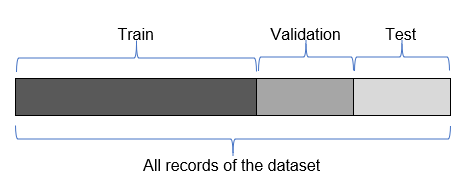
You can also find papers with splitting only for train/test. In this case test means validation.

---

26.2 Splitting data in R

Lets describe some conditions before start studiyng splitting data functions in R:

• We will use same seed for all splittings to control results reproduction, for example, let it be 2021.
• We will use dataset for client churn prediction Telco Customer Churn: https://www.kaggle.com/blastchar/telco-customer-churn

Short dataset description:

• customerID - Customer ID
• gender Whether the customer is a male or a female
• SeniorCitizen - Whether the customer is a senior citizen or not (1, 0)
• Partner - Whether the customer has a partner or not (Yes, No)
• Dependents - Whether the customer has dependents or not (Yes, No)
• tenure - Number of months the customer has stayed with the company
• PhoneService - Whether the customer has a phone service or not (Yes, No)
• MultipleLines - Whether the customer has multiple lines or not (Yes, No, No phone service)
• InternetService - Customer’s internet service provider (DSL, Fiber optic, No)
• OnlineSecurity - Whether the customer has online security or not (Yes, No, No internet service)
• OnlineBackup - Whether the customer has online backup or not (Yes, No, No internet service)
• DeviceProtection - Whether the customer has device protection or not (Yes, No, No internet service)
• TechSupport - Whether the customer has tech support or not (Yes, No, No internet service)
• StreamingTV - Whether the customer has streaming TV or not (Yes, No, No internet service)
• StreamingMovies - Whether the customer has streaming movies or not (Yes, No, No internet service)
• Contract - The contract term of the customer (Month-to-month, One year, Two year)
• PaperlessBilling - Whether the customer has paperless billing or not (Yes, No)
• PaymentMethod - The customer’s payment method (Electronic check, Mailed check, Bank transfer (automatic), Credit card (automatic))
• MonthlyCharges - The amount charged to the customer monthly
• TotalCharges - The total amount charged to the customer
• Churn - Whether the customer churned or not (Yes or No)

# read data
telecom_users <- read.csv("data/telecom_users.csv")
head(telecom_users)

A data.frame: 6 × 22

	X	customerID	gender	SeniorCitizen	Partner	Dependents	tenure	PhoneService	MultipleLines	InternetService	⋯	DeviceProtection	TechSupport	StreamingTV	StreamingMovies	Contract	PaperlessBilling	PaymentMethod	MonthlyCharges	TotalCharges	Churn
	<int>	<chr>	<chr>	<int>	<chr>	<chr>	<int>	<chr>	<chr>	<chr>	⋯	<chr>	<chr>	<chr>	<chr>	<chr>	<chr>	<chr>	<chr>	<dbl>	<chr>
1	1869	7010-BRBUU	Male	0	Yes	Yes	72	Yes	Yes	No	⋯	No internet service	No internet service	No internet service	No internet service	Two year	No	Credit card (automatic)	24.1	1734.65	No
2	4528	9688-YGXVR	Female	0	No	No	44	Yes	No	Fiber optic	⋯	Yes	No	Yes	No	Month-to-month	Yes	Credit card (automatic)	88.15	3973.20	No
3	6344	9286-DOJGF	Female	1	Yes	No	38	Yes	Yes	Fiber optic	⋯	No	No	No	No	Month-to-month	Yes	Bank transfer (automatic)	74.95	2869.85	Yes
4	6739	6994-KERXL	Male	0	No	No	4	Yes	No	DSL	⋯	No	No	No	Yes	Month-to-month	Yes	Electronic check	55.9	238.50	No
5	432	2181-UAESM	Male	0	No	No	2	Yes	No	DSL	⋯	Yes	No	No	No	Month-to-month	No	Electronic check	53.45	119.50	No
6	2215	4312-GVYNH	Female	0	Yes	No	70	No	No phone service	DSL	⋯	Yes	Yes	No	Yes	Two year	Yes	Bank transfer (automatic)	49.85	3370.20	No

Lets check the proportion of column Churn == Yes and Churn == No in dataset with CrossTable() function from gmodels package.

# install.packages("gmodels")

library(gmodels)
CrossTable(telecom_users$Churn)

 
   Cell Contents
|-------------------------|
|                       N |
|         N / Table Total |
|-------------------------|

 
Total Observations in Table:  5986 

 
          |        No |       Yes | 
          |-----------|-----------|
          |      4399 |      1587 | 
          |     0.735 |     0.265 | 
          |-----------|-----------|



 

You can also use CrossTable() to check cross proportions by other fields. Lets check crosstable for TechSupport and Churn:

CrossTable(telecom_users$Churn, telecom_users$TechSupport) # for example

 
   Cell Contents
|-------------------------|
|                       N |
| Chi-square contribution |
|           N / Row Total |
|           N / Col Total |
|         N / Table Total |
|-------------------------|

 
Total Observations in Table:  5986 

 
                    | telecom_users$TechSupport 
telecom_users$Churn |                  No | No internet service |                 Yes |           Row Total | 
--------------------|---------------------|---------------------|---------------------|---------------------|
                 No |                1738 |                1192 |                1469 |                4399 | 
                    |              87.892 |              62.377 |              29.512 |                     | 
                    |               0.395 |               0.271 |               0.334 |               0.735 | 
                    |               0.587 |               0.923 |               0.847 |                     | 
                    |               0.290 |               0.199 |               0.245 |                     | 
--------------------|---------------------|---------------------|---------------------|---------------------|
                Yes |                1222 |                  99 |                 266 |                1587 | 
                    |             243.627 |             172.904 |              81.805 |                     | 
                    |               0.770 |               0.062 |               0.168 |               0.265 | 
                    |               0.413 |               0.077 |               0.153 |                     | 
                    |               0.204 |               0.017 |               0.044 |                     | 
--------------------|---------------------|---------------------|---------------------|---------------------|
       Column Total |                2960 |                1291 |                1735 |                5986 | 
                    |               0.494 |               0.216 |               0.290 |                     | 
--------------------|---------------------|---------------------|---------------------|---------------------|

 

You can see that most part of Churn 1222 of 1587

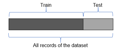
Next, we will check 6 possible ways to split data for train/test sets.

---

26.2.1 Split with sample()

sample_size = round(nrow(telecom_users)*.70) # setting what is 70%
print(paste0("Size: ", sample_size))

index <- sample(nrow(telecom_users), size = sample_size)
 
train <- telecom_users[index, ] # index is numbers of selected rows from dataset
test <-telecom_users[-index, ] # -index select only rows not in index

[1] "Size: 4190"

# check Churn == Yes/No proportion in train/test
CrossTable(train$Churn)

 
   Cell Contents
|-------------------------|
|                       N |
|         N / Table Total |
|-------------------------|

 
Total Observations in Table:  4190 

 
          |        No |       Yes | 
          |-----------|-----------|
          |      3074 |      1116 | 
          |     0.734 |     0.266 | 
          |-----------|-----------|



 

# check Churn == Yes/No proportion in train/test
CrossTable(test$Churn)

 
   Cell Contents
|-------------------------|
|                       N |
|         N / Table Total |
|-------------------------|

 
Total Observations in Table:  1796 

 
          |        No |       Yes | 
          |-----------|-----------|
          |      1325 |       471 | 
          |     0.738 |     0.262 | 
          |-----------|-----------|



 

Its 0.260 for train and 0.276 for test. Diffrence is 1,6%, so, its close.

---

26.2.2 Split with sample_frac from dplyr

library(dplyr)
set.seed(2023)

# Using the above function to create 70 - 30 slipt into test and train

tu <- telecom_users %>% mutate(Id = row_number())

train <- tu %>% sample_frac(.70)
test <- tu[-train$Id, ]

Attaching package: 'dplyr'


The following objects are masked from 'package:stats':

    filter, lag


The following objects are masked from 'package:base':

    intersect, setdiff, setequal, union

nrow(train)

4190

# check Churn == Yes/No proportion in train/test
CrossTable(train$Churn)
CrossTable(test$Churn)

 
   Cell Contents
|-------------------------|
|                       N |
|         N / Table Total |
|-------------------------|

 
Total Observations in Table:  4190 

 
          |        No |       Yes | 
          |-----------|-----------|
          |      3099 |      1091 | 
          |     0.740 |     0.260 | 
          |-----------|-----------|



 

 
   Cell Contents
|-------------------------|
|                       N |
|         N / Table Total |
|-------------------------|

 
Total Observations in Table:  1796 

 
          |        No |       Yes | 
          |-----------|-----------|
          |      1300 |       496 | 
          |     0.724 |     0.276 | 
          |-----------|-----------|



 

sample_n made other proportion of Churn == Yes/No and difference just 0.7%.

---

26.2.3 Split with createDataPartition() from caret

#install.packages("caret")

Updating HTML index of packages in '.Library'

Making 'packages.html' ...
 done

library(caret)
set.seed(2023)
 
index = createDataPartition(telecom_users$Churn, p = 0.70, list = FALSE)
train = telecom_users[index, ]
test = telecom_users[-index, ]

Loading required package: ggplot2

Loading required package: lattice

# check Churn == Yes/No proportion in train/test
CrossTable(train$Churn)
CrossTable(test$Churn)

 
   Cell Contents
|-------------------------|
|                       N |
|         N / Table Total |
|-------------------------|

 
Total Observations in Table:  4191 

 
          |        No |       Yes | 
          |-----------|-----------|
          |      3080 |      1111 | 
          |     0.735 |     0.265 | 
          |-----------|-----------|



 

 
   Cell Contents
|-------------------------|
|                       N |
|         N / Table Total |
|-------------------------|

 
Total Observations in Table:  1795 

 
          |        No |       Yes | 
          |-----------|-----------|
          |      1319 |       476 | 
          |     0.735 |     0.265 | 
          |-----------|-----------|



 

Ckeck the proportion of target variable. Caret trying to make the same split for both train and test. This is one of the best split methods in R.

---

26.2.4 Split with sample.split from caTools

#install.packages("caTools")

library(caTools)
 
set.seed(2023)
sample = sample.split(telecom_users$Churn, SplitRatio = .70)

train = telecom_users[sample, ]
test  = telecom_users[!sample, ]

# check Churn == Yes/No proportion in train/test
CrossTable(train$Churn)
CrossTable(test$Churn)

 
   Cell Contents
|-------------------------|
|                       N |
|         N / Table Total |
|-------------------------|

 
Total Observations in Table:  4190 

 
          |        No |       Yes | 
          |-----------|-----------|
          |      3079 |      1111 | 
          |     0.735 |     0.265 | 
          |-----------|-----------|



 

 
   Cell Contents
|-------------------------|
|                       N |
|         N / Table Total |
|-------------------------|

 
Total Observations in Table:  1796 

 
          |        No |       Yes | 
          |-----------|-----------|
          |      1320 |       476 | 
          |     0.735 |     0.265 | 
          |-----------|-----------|



 

---

Для нашого курсу це не потрібно поки! Переходимо до наступної теми. Цей матеріал в детелях буде розглянуто під час вивчення крос-валідації.

26.3 Splitting for n-folds

# read data again
library(caret)
telecom_users <- read.csv("../../data/telecom_users.csv")
nrow(telecom_users)
head(telecom_users)

5986

A data.frame: 6 × 22

	X	customerID	gender	SeniorCitizen	Partner	Dependents	tenure	PhoneService	MultipleLines	InternetService	...	DeviceProtection	TechSupport	StreamingTV	StreamingMovies	Contract	PaperlessBilling	PaymentMethod	MonthlyCharges	TotalCharges	Churn
	<int>	<chr>	<chr>	<int>	<chr>	<chr>	<int>	<chr>	<chr>	<chr>	...	<chr>	<chr>	<chr>	<chr>	<chr>	<chr>	<chr>	<chr>	<dbl>	<chr>
1	1869	7010-BRBUU	Male	0	Yes	Yes	72	Yes	Yes	No	...	No internet service	No internet service	No internet service	No internet service	Two year	No	Credit card (automatic)	24.1	1734.65	No
2	4528	9688-YGXVR	Female	0	No	No	44	Yes	No	Fiber optic	...	Yes	No	Yes	No	Month-to-month	Yes	Credit card (automatic)	88.15	3973.20	No
3	6344	9286-DOJGF	Female	1	Yes	No	38	Yes	Yes	Fiber optic	...	No	No	No	No	Month-to-month	Yes	Bank transfer (automatic)	74.95	2869.85	Yes
4	6739	6994-KERXL	Male	0	No	No	4	Yes	No	DSL	...	No	No	No	Yes	Month-to-month	Yes	Electronic check	55.9	238.50	No
5	432	2181-UAESM	Male	0	No	No	2	Yes	No	DSL	...	Yes	No	No	No	Month-to-month	No	Electronic check	53.45	119.50	No
6	2215	4312-GVYNH	Female	0	Yes	No	70	No	No phone service	DSL	...	Yes	Yes	No	Yes	Two year	Yes	Bank transfer (automatic)	49.85	3370.20	No

folds <- createFolds(telecom_users)
folds

$Fold01

1. 1
2. 10

$Fold02

1. 3
2. 4
3. 15

$Fold03

1. 2
2. 17

$Fold04

8

$Fold05

1. 16
2. 22

$Fold06

1. 9
2. 18

$Fold07

1. 19
2. 20

$Fold08

1. 5
2. 12
3. 14

$Fold09

11

$Fold10

1. 6
2. 7
3. 13
4. 21

#library(caret)
#library(mlbench)
#data(Sonar)
 
#folds <- createFolds(Sonar$Class)
#str(folds)

---

26.4 References

1. About Train, Validation and Test Sets in Machine Learning by Tarang Shah. Url: https://towardsdatascience.com/train-validation-and-test-sets-72cb40cba9e7