1  Woe Binning

2 Woe Binning

Курс: “Матетичне моделювання в R”

---

# install.packages("openxlsx")

Sys.setlocale("LC_CTYPE", "ukrainian")
options(warn = -1)

'Ukrainian_Ukraine.1251'

2.1 Набір даних

Джерело: https://github.com/gastonstat/CreditScoring/blob/master/CleanCreditScoring.csv

Завантажимо дані:

library(openxlsx)
data <- openxlsx::read.xlsx("data/CreditScoring.xlsx", sheet = 1, startRow = 1, colNames = TRUE, rowNames = FALSE)
str(data)

'data.frame':   4446 obs. of  16 variables:
 $ Status   : chr  "good" "good" "bad" "good" ...
 $ Seniority: num  9 17 10 0 0 1 29 9 0 0 ...
 $ Home     : chr  "rent" "rent" "owner" "rent" ...
 $ Time     : num  60 60 36 60 36 60 60 12 60 48 ...
 $ Age      : num  30 58 46 24 26 36 44 27 32 41 ...
 $ Marital  : chr  "married" "widow" "married" "single" ...
 $ Records  : chr  "no_rec" "no_rec" "yes_rec" "no_rec" ...
 $ Job      : chr  "freelance" "fixed" "freelance" "fixed" ...
 $ Expenses : num  73 48 90 63 46 75 75 35 90 90 ...
 $ Income   : num  129 131 200 182 107 214 125 80 107 80 ...
 $ Assets   : num  0 0 3000 2500 0 3500 10000 0 15000 0 ...
 $ Debt     : num  0 0 0 0 0 0 0 0 0 0 ...
 $ Amount   : num  800 1000 2000 900 310 650 1600 200 1200 1200 ...
 $ Price    : num  846 1658 2985 1325 910 ...
 $ Finrat   : num  94.6 60.3 67 67.9 34.1 ...
 $ Savings  : num  4.2 4.98 1.98 7.93 7.08 ...

Опишемо дані:

• Status - credit status (Target)
• Seniority job seniority (years)
• Home type of home ownership
• Time time of requested loan
• Age client’s age
• Marital marital status
• Records existance of records
• Job type of job
• Expenses amount of expenses
• Income amount of income
• Assets amount of assets
• Debt amount of debt
• Amount amount requested of loan
• Price price of good

---

2.2 Простий бінінг змінних

2.2.1 Категоріальна змінна

Створимо дата-фрейм для зберігання інформації про групи змінної Home (як приклад біннігу категоріального показника):

home_groups <- data.frame(Group = unique(data$Home), 
                          Good = c(0), Bad = c(0), 
                          GoodP = c(0), BadP = c(0),
                          WOE = c(0), IV = c(0))
home_groups

A data.frame: 6 × 7

Group	Good	Bad	GoodP	BadP	WOE	IV
<chr>	<dbl>	<dbl>	<dbl>	<dbl>	<dbl>	<dbl>
rent	0	0	0	0	0	0
owner	0	0	0	0	0	0
parents	0	0	0	0	0	0
priv	0	0	0	0	0	0
other	0	0	0	0	0	0
ignore	0	0	0	0	0	0

Переглянемо можливі варіанти показника Status, який є залежною бінарною змінною поточної задачі:

library(gmodels)
CrossTable(data$Status)

 
   Cell Contents
|-------------------------|
|                       N |
|         N / Table Total |
|-------------------------|

 
Total Observations in Table:  4446 

 
          |       bad |      good | 
          |-----------|-----------|
          |      1249 |      3197 | 
          |     0.281 |     0.719 | 
          |-----------|-----------|



 

Сформуємо групи та обчислимо значення по кожній групі:

for(i in 1:nrow(home_groups)) {
  
  group <- home_groups$Group[i]
  
  home_groups$Good[i] <- nrow(data[data$Home == group & data$Status == "good", ])
  home_groups$Bad[i] <- nrow(data[data$Home == group & data$Status == "bad", ])
  
  home_groups$GoodP[i] <- home_groups$Good[i]/nrow(data[data$Status == "good", ])
  home_groups$BadP[i] <- home_groups$Bad[i]/nrow(data[data$Status == "bad", ])
  
  home_groups$WOE[i] <- log( home_groups$GoodP[i] / home_groups$BadP[i])
  home_groups$IV[i] <- (home_groups$GoodP[i] - home_groups$BadP[i])*home_groups$WOE[i]
}

home_groups

A data.frame: 6 × 7

Group	Good	Bad	GoodP	BadP	WOE	IV
<chr>	<dbl>	<dbl>	<dbl>	<dbl>	<dbl>	<dbl>
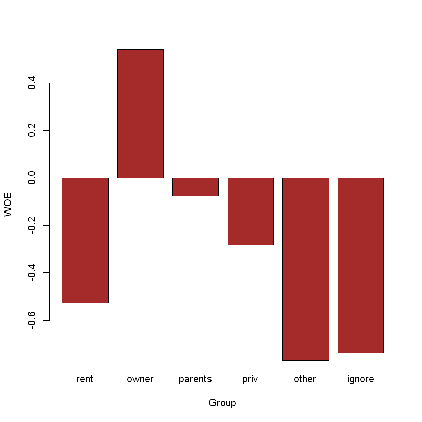
rent	585	388	0.182984048	0.310648519	-0.52926313	0.067568098
owner	1716	390	0.536753206	0.312249800	0.54173490	0.121621331
parents	550	232	0.172036284	0.185748599	-0.07668873	0.001051580
priv	162	84	0.050672505	0.067253803	-0.28309010	0.004694001
other	173	146	0.054113231	0.116893515	-0.77018467	0.048352412
ignore	11	9	0.003440726	0.007205765	-0.73919894	0.002783113

Переглянемо сумарний IV:

home_iv <- sum(home_groups$IV)
home_iv

0.246070534510342

Візуалізуємо групи:

barplot(home_groups$WOE, 
        col="brown", 
        names.arg=c(as.character(home_groups$Group)), 
        xlab="Group",
        ylab="WOE"
)

Створимо датафрейм для нових WOE-даних:

new_df <- data.frame(Status = data$Status, Home = data$Home, HomeWoe = c(0))

Замінимо значення на WOE:

for(i in 1:nrow(home_groups)) {
  group <- home_groups$Group[i]
  woe <- home_groups$WOE[i]  
  new_df[new_df$Home == group, ]$HomeWoe <- woe
}

tail(new_df)

A data.frame: 6 × 3

	Status	Home	HomeWoe
	<chr>	<chr>	<dbl>
4441	bad	other	-0.7701847
4442	bad	rent	-0.5292631
4443	good	owner	0.5417349
4444	bad	owner	0.5417349
4445	good	rent	-0.5292631
4446	good	owner	0.5417349

---

2.2.2 Числова змінна

Обрахуємо приклад числовиго показника (на прикладі Age):

min_age <- min(data$Age)
max_age <- max(data$Age)

step <- round(max_age - min_age)/10


age_groups <- data.frame(Min = seq(min_age, max_age-step, step), 
                         Max = seq(min_age + step, max_age, step), 
                          Good = c(0), Bad = c(0), 
                          GoodP = c(0), BadP = c(0),
                          WOE = c(0), IV = c(0))

age_groups

A data.frame: 10 × 8

Min	Max	Good	Bad	GoodP	BadP	WOE	IV
<dbl>	<dbl>	<dbl>	<dbl>	<dbl>	<dbl>	<dbl>	<dbl>
18	23	0	0	0	0	0	0
23	28	0	0	0	0	0	0
28	33	0	0	0	0	0	0
33	38	0	0	0	0	0	0
38	43	0	0	0	0	0	0
43	48	0	0	0	0	0	0
48	53	0	0	0	0	0	0
53	58	0	0	0	0	0	0
58	63	0	0	0	0	0	0
63	68	0	0	0	0	0	0

Сформуємо групи:

for(i in 1:nrow(age_groups)) {
  
  min <- age_groups$Min[i]
  max<- age_groups$Max[i]
  
  age_groups$Good[i] <- nrow(data[data$Age >= min & data$Age < max & data$Status == "good", ])
  age_groups$Bad[i] <- nrow(data[data$Age >= min & data$Age < max & data$Status == "bad", ])
  
  if(i == nrow(age_groups)) {
    age_groups$Good[i] <- age_groups$Good[i] + nrow(data[data$Age == max & data$Status == "good", ])
    age_groups$Bad[i] <- age_groups$Bad[i] + nrow(data[data$Age == max & data$Status == "bad", ])
  }
  
  age_groups$GoodP[i] <- age_groups$Good[i]/nrow(data[data$Status == "good", ])
  age_groups$BadP[i] <- age_groups$Bad[i]/nrow(data[data$Status == "bad", ])
  
  age_groups$WOE[i] <- log( age_groups$GoodP[i] / age_groups$BadP[i])
  
  age_groups$IV[i] <- (age_groups$GoodP[i] - age_groups$BadP[i]) * age_groups$WOE[i]
}

age_groups

A data.frame: 10 × 8

Min	Max	Good	Bad	GoodP	BadP	WOE	IV
<dbl>	<dbl>	<dbl>	<dbl>	<dbl>	<dbl>	<dbl>	<dbl>
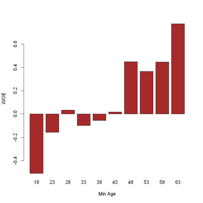
18	23	169	110	0.05286206	0.088070456	-0.51045129	0.0179721723
23	28	505	231	0.15796059	0.184947958	-0.15772892	0.0042566888
28	33	564	213	0.17641539	0.170536429	0.03389245	0.0001992523
33	38	491	212	0.15358148	0.169735789	-0.10001179	0.0016156210
38	43	443	183	0.13856741	0.146517214	-0.05578602	0.0004434881
43	48	320	123	0.10009384	0.098478783	0.01626700	0.0000262721
48	53	317	79	0.09915546	0.063250600	0.44958428	0.0161422597
53	58	214	58	0.06693775	0.046437150	0.36566337	0.0074963200
58	63	124	31	0.03878636	0.024819856	0.44642472	0.0062349937
63	68	50	9	0.01563966	0.007205765	0.77492879	0.0065356700

Сумарний IV:

age_iv <- sum(age_groups$IV)
age_iv

0.0609227380464588

Візуалізуємо значення груп WOE:

barplot(age_groups$WOE, 
        col="brown", 
        names.arg=c(age_groups$Min), 
        xlab="Min Age",
        ylab="WOE"
)

Замінимо значення на WOE:

new_df$Age <- data$Age
new_df$AgeWoe <- c(0)

for(i in 1:nrow(age_groups)) {
  
  min <- age_groups$Min[i]
  max <- age_groups$Max[i]
  woe <- age_groups$WOE[i]
  
  new_df[new_df$Age >= min & new_df$Age < max, ]$AgeWoe <- woe
  
  if(i == nrow(age_groups)) {
    new_df$AgeWoe[i] <- woe
  }
  
}

head(new_df)

A data.frame: 6 × 5

	Status	Home	HomeWoe	Age	AgeWoe
	<chr>	<chr>	<dbl>	<dbl>	<dbl>
1	good	rent	-0.5292631	30	0.03389245
2	good	rent	-0.5292631	58	0.44642472
3	bad	owner	0.5417349	46	0.01626700
4	good	rent	-0.5292631	24	-0.15772892
5	good	rent	-0.5292631	26	-0.15772892
6	good	owner	0.5417349	36	-0.10001179

Видалимо оригінальні значення з набору даних:

new_df$Home <- NULL
new_df$Age <- NULL
head(new_df)

A data.frame: 6 × 3

	Status	HomeWoe	AgeWoe
	<chr>	<dbl>	<dbl>
1	good	-0.5292631	0.03389245
2	good	-0.5292631	0.44642472
3	bad	0.5417349	0.01626700
4	good	-0.5292631	-0.15772892
5	good	-0.5292631	-0.15772892
6	good	0.5417349	-0.10001179

---

2.3 Бінінг з використанням woeBin

---

2.4 Бінінг з використанням rBin

---

2.5 Бінінг з використанням smbinning

---

2.6 Бінінг з використанням scorecard

---