5  Нейронні мережі. Регресія. Вартість житла

Курс: “Математичне моделювання в R”

---

У цій лекції ми скористаємося набором даних Boston: вартість житла у пригородах Бостона

5.1 Dataset description

# install.packages("MASS")
# install.packages("neuralnet")
# install.packages("clusterGeneration")
# install.packages("devtools")
# install.packages("caTools")
# install.packages("reshape")
# install.packages("Metrics")
# install.packages("nnet")
#install.packages("plyr")
#install.packages("boot")

medv is TARGET!

library(MASS)
?Boston

Boston {MASS}

R Documentation

Housing Values in Suburbs of Boston

Description

The Boston data frame has 506 rows and 14 columns.

Usage

Boston

Format

This data frame contains the following columns:

crim

per capita crime rate by town.

zn

proportion of residential land zoned for lots over 25,000 sq.ft.

indus

proportion of non-retail business acres per town.

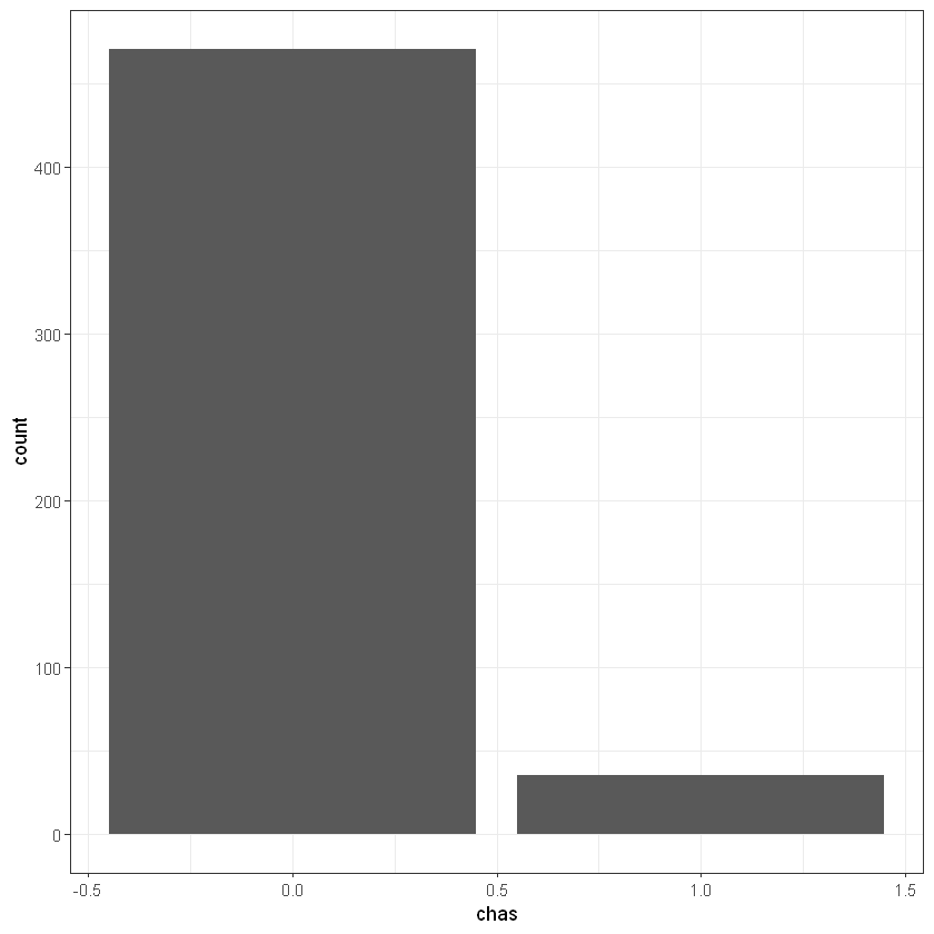
chas

Charles River dummy variable (= 1 if tract bounds river; 0 otherwise).

nox

nitrogen oxides concentration (parts per 10 million).

rm

average number of rooms per dwelling.

age

proportion of owner-occupied units built prior to 1940.

dis

weighted mean of distances to five Boston employment centres.

rad

index of accessibility to radial highways.

tax

full-value property-tax rate per $10,000.

ptratio

pupil-teacher ratio by town.

black

1000(Bk - 0.63)^2 where Bk is the proportion of blacks by town.

lstat

lower status of the population (percent).

medv

median value of owner-occupied homes in $1000s.

Source

Harrison, D. and Rubinfeld, D.L. (1978) Hedonic prices and the demand for clean air. J. Environ. Economics and Management 5, 81–102.

Belsley D.A., Kuh, E. and Welsch, R.E. (1980) Regression Diagnostics. Identifying Influential Data and Sources of Collinearity. New York: Wiley.

---

[Package MASS version 7.3-58.1 ]

Переглянемо дані:

head(Boston)

A data.frame: 6 × 14

	crim	zn	indus	chas	nox	rm	age	dis	rad	tax	ptratio	black	lstat	medv
	<dbl>	<dbl>	<dbl>	<int>	<dbl>	<dbl>	<dbl>	<dbl>	<int>	<dbl>	<dbl>	<dbl>	<dbl>	<dbl>
1	0.00632	18	2.31	0	0.538	6.575	65.2	4.0900	1	296	15.3	396.90	4.98	24.0
2	0.02731	0	7.07	0	0.469	6.421	78.9	4.9671	2	242	17.8	396.90	9.14	21.6
3	0.02729	0	7.07	0	0.469	7.185	61.1	4.9671	2	242	17.8	392.83	4.03	34.7
4	0.03237	0	2.18	0	0.458	6.998	45.8	6.0622	3	222	18.7	394.63	2.94	33.4
5	0.06905	0	2.18	0	0.458	7.147	54.2	6.0622	3	222	18.7	396.90	5.33	36.2
6	0.02985	0	2.18	0	0.458	6.430	58.7	6.0622	3	222	18.7	394.12	5.21	28.7

str(Boston)

'data.frame':   506 obs. of  14 variables:
 $ crim   : num  0.00632 0.02731 0.02729 0.03237 0.06905 ...
 $ zn     : num  18 0 0 0 0 0 12.5 12.5 12.5 12.5 ...
 $ indus  : num  2.31 7.07 7.07 2.18 2.18 2.18 7.87 7.87 7.87 7.87 ...
 $ chas   : int  0 0 0 0 0 0 0 0 0 0 ...
 $ nox    : num  0.538 0.469 0.469 0.458 0.458 0.458 0.524 0.524 0.524 0.524 ...
 $ rm     : num  6.58 6.42 7.18 7 7.15 ...
 $ age    : num  65.2 78.9 61.1 45.8 54.2 58.7 66.6 96.1 100 85.9 ...
 $ dis    : num  4.09 4.97 4.97 6.06 6.06 ...
 $ rad    : int  1 2 2 3 3 3 5 5 5 5 ...
 $ tax    : num  296 242 242 222 222 222 311 311 311 311 ...
 $ ptratio: num  15.3 17.8 17.8 18.7 18.7 18.7 15.2 15.2 15.2 15.2 ...
 $ black  : num  397 397 393 395 397 ...
 $ lstat  : num  4.98 9.14 4.03 2.94 5.33 ...
 $ medv   : num  24 21.6 34.7 33.4 36.2 28.7 22.9 27.1 16.5 18.9 ...

5.2 Data visualization

Lets move our dataset to special variable:

data <- Boston
head(data)

A data.frame: 6 × 14

	crim	zn	indus	chas	nox	rm	age	dis	rad	tax	ptratio	black	lstat	medv
	<dbl>	<dbl>	<dbl>	<int>	<dbl>	<dbl>	<dbl>	<dbl>	<int>	<dbl>	<dbl>	<dbl>	<dbl>	<dbl>
1	0.00632	18	2.31	0	0.538	6.575	65.2	4.0900	1	296	15.3	396.90	4.98	24.0
2	0.02731	0	7.07	0	0.469	6.421	78.9	4.9671	2	242	17.8	396.90	9.14	21.6
3	0.02729	0	7.07	0	0.469	7.185	61.1	4.9671	2	242	17.8	392.83	4.03	34.7
4	0.03237	0	2.18	0	0.458	6.998	45.8	6.0622	3	222	18.7	394.63	2.94	33.4
5	0.06905	0	2.18	0	0.458	7.147	54.2	6.0622	3	222	18.7	396.90	5.33	36.2
6	0.02985	0	2.18	0	0.458	6.430	58.7	6.0622	3	222	18.7	394.12	5.21	28.7

Let’s check a correlation between parameters:

suppressMessages(library(corrplot))
corrplot(cor(data))

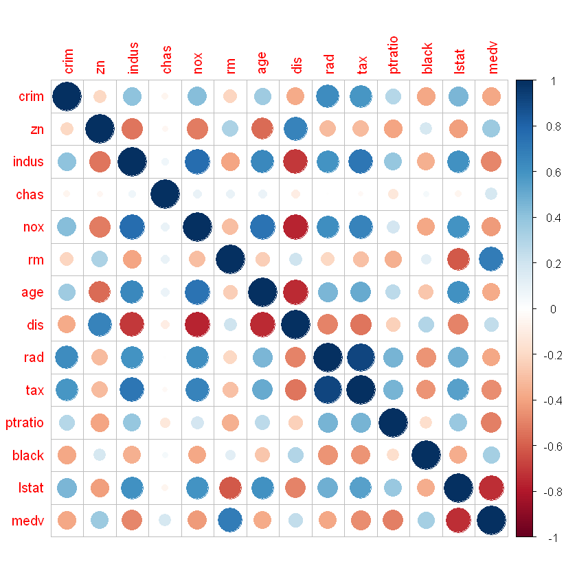
Rad and tax has highest correlation: 0.91

• rad - index of accessibility to radial highways.
• tax - full-value property-tax rate per $10,000.

library(ggplot2)

ggplot(data, aes(medv)) + 
    geom_histogram(bins = 25, alpha = 0.5, fill = 'blue', color='black')  + 
    theme_bw()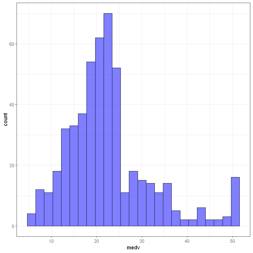

#crim
ggplot(data, aes(crim)) + 
    geom_histogram(bins = 25, alpha = 0.5, fill = 'blue', color='black')  + 
    theme_bw()

#zn
ggplot(data, aes(zn)) + 
    geom_histogram(bins = 25, alpha = 0.5, fill = 'blue', color='black')  + 
    theme_bw()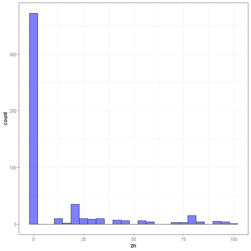

#indus
ggplot(data, aes(indus)) + 
    geom_histogram(bins = 25, alpha = 0.5, fill = 'blue', color='black')  + 
    theme_bw()

#chas 
ggplot(data, aes(chas)) + 
    geom_bar(aes(fill = chas)) + 
    theme_bw()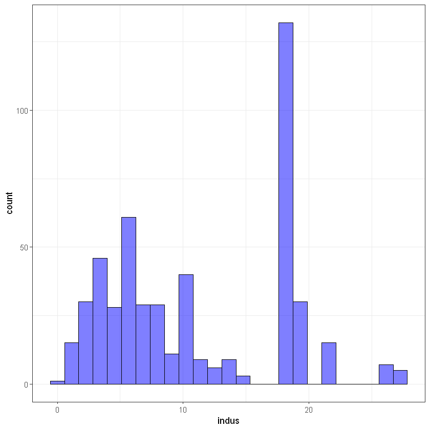

# nox
ggplot(data, aes(nox)) + 
    geom_histogram(bins = 10, alpha = 0.5, fill = 'blue', color='black')  + 
    theme_bw()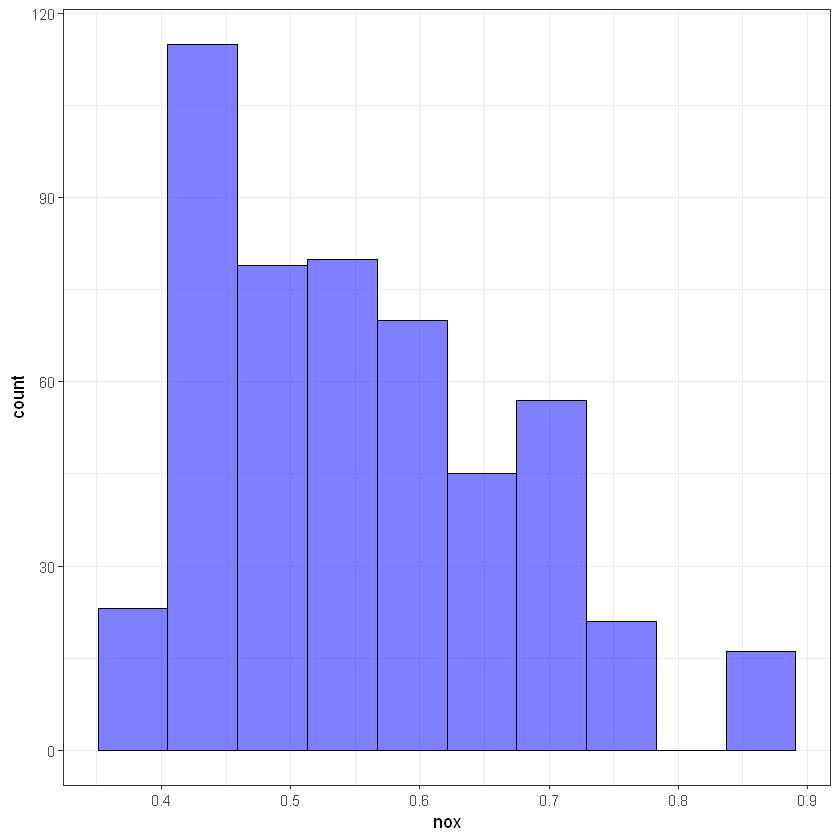

# rm
ggplot(data, aes(rm)) + 
    geom_histogram(bins = 10, alpha = 0.5, fill = 'blue', color='black')  + 
    theme_bw()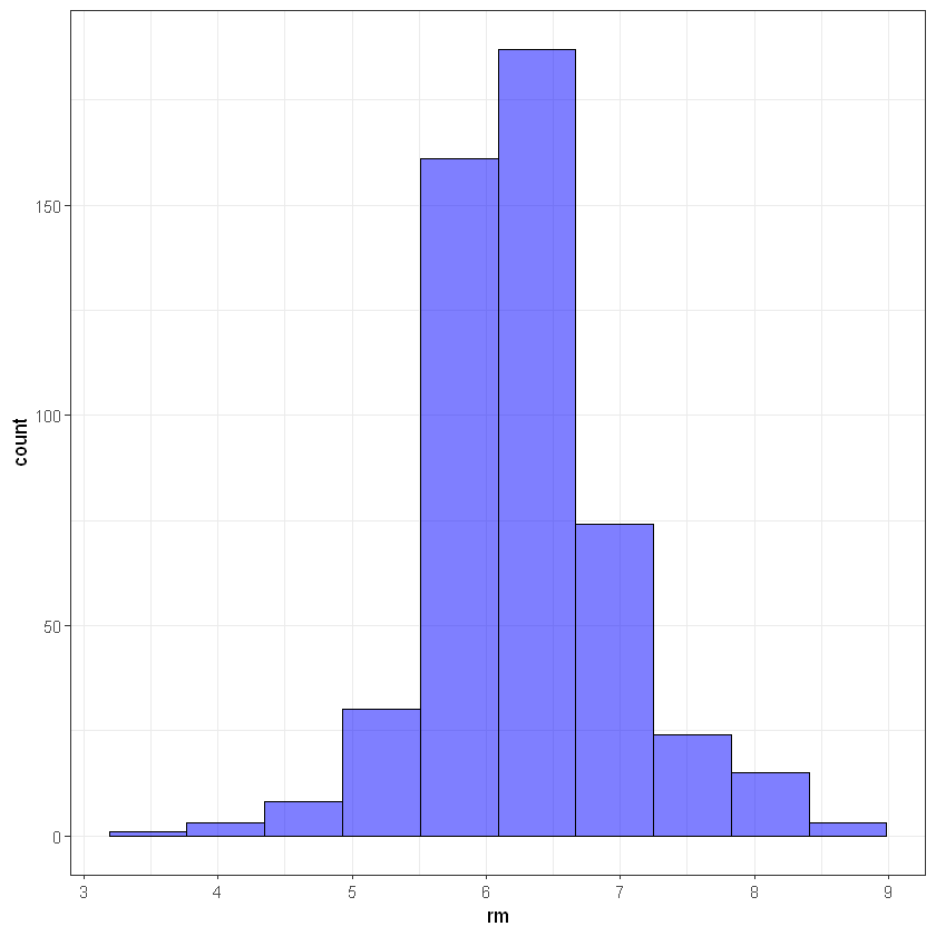

# age
ggplot(data, aes(age)) + 
    geom_histogram(bins = 15, alpha = 0.5, fill = 'blue', color='black')  + 
    theme_bw()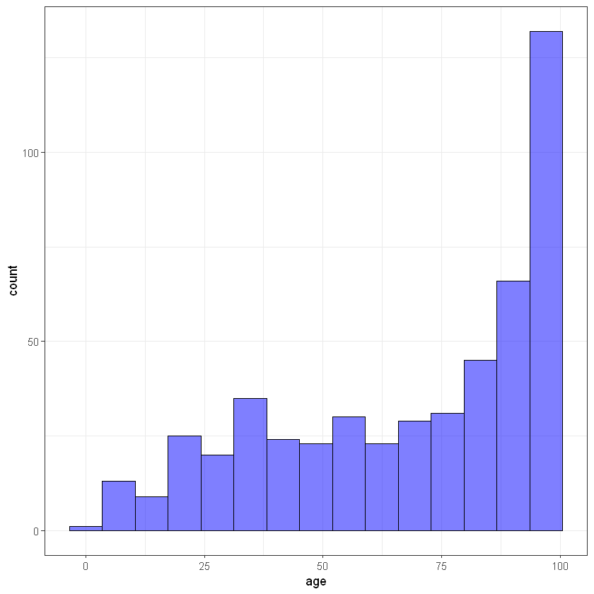

# dis
ggplot(data, aes(dis)) + 
    geom_histogram(bins = 15, alpha = 0.5, fill = 'blue', color='black')  + 
    theme_bw()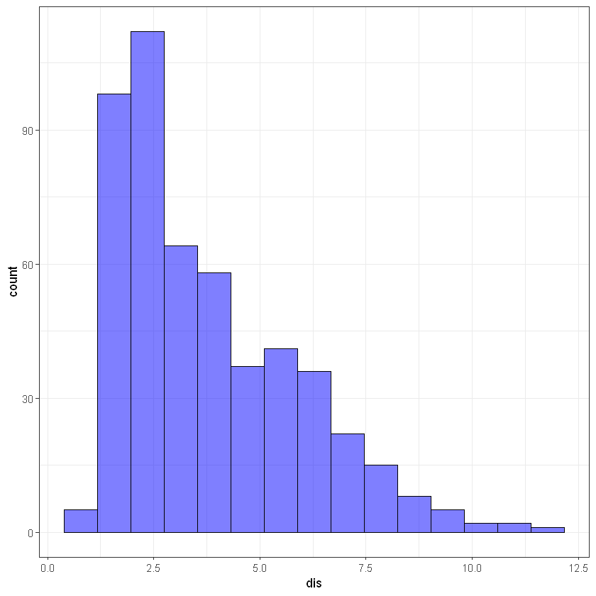

#rad
ggplot(data, aes(ptratio)) + 
    geom_histogram(bins = 10, alpha = 0.5, fill = 'blue', color='black')  + 
    theme_bw()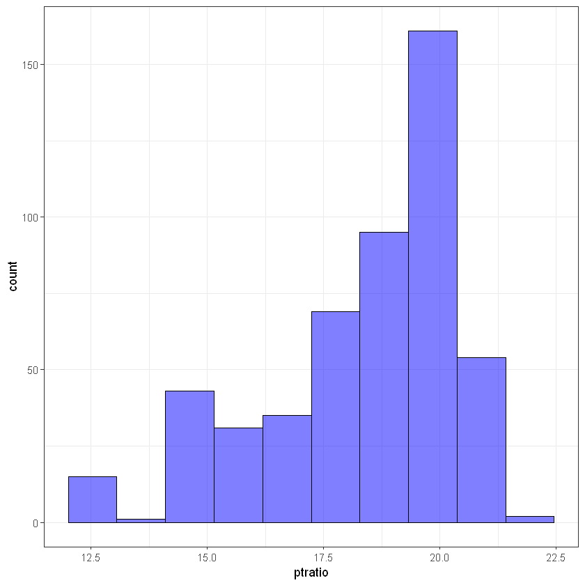

# black
ggplot(data, aes(black)) + 
    geom_histogram(bins = 10, alpha = 0.5, fill = 'blue', color='black')  + 
    theme_bw()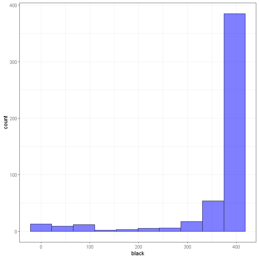

# lstat
ggplot(data, aes(lstat)) + 
    geom_histogram(bins = 25, alpha = 0.5, fill = 'blue', color='black')  + 
    theme_bw()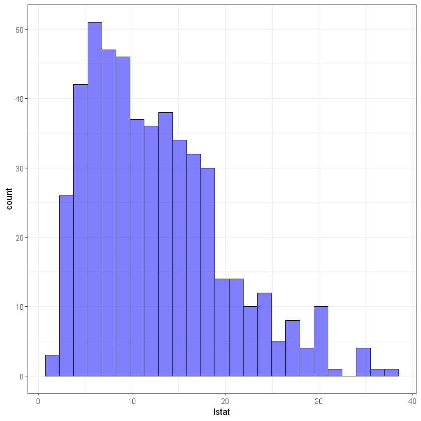

# nox
ggplot(data, aes(nox)) + 
    geom_histogram(bins = 25, alpha = 0.5, fill = 'blue', color='black')  + 
    theme_bw()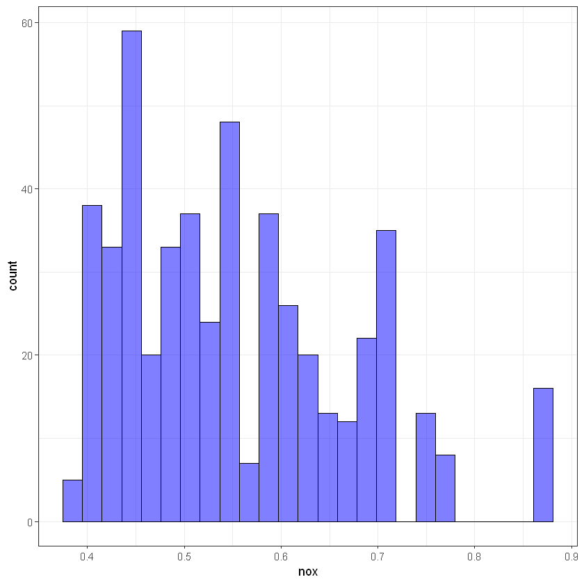

---

5.3 Data scaling

Для роботи з нейромережами хорошою практикою є нормалізація даних перед використанням. Скористаємося формулою \((X-Xmin)/(Xmax-Xmin)\).

Визначимо мінімальні та максимальні значення по факторах:

suppressMessages(library(dplyr))

normalizeData <- function(x) {
    return ((x - min(x)) / (max(x) - min(x)))
}

revertData <- function(scaled, original) {
    return (scaled * (max(original) - min(original)) + min(original))    
}

data %>% head()

A data.frame: 6 × 14

	crim	zn	indus	chas	nox	rm	age	dis	rad	tax	ptratio	black	lstat	medv
	<dbl>	<dbl>	<dbl>	<int>	<dbl>	<dbl>	<dbl>	<dbl>	<int>	<dbl>	<dbl>	<dbl>	<dbl>	<dbl>
1	0.00632	18	2.31	0	0.538	6.575	65.2	4.0900	1	296	15.3	396.90	4.98	24.0
2	0.02731	0	7.07	0	0.469	6.421	78.9	4.9671	2	242	17.8	396.90	9.14	21.6
3	0.02729	0	7.07	0	0.469	7.185	61.1	4.9671	2	242	17.8	392.83	4.03	34.7
4	0.03237	0	2.18	0	0.458	6.998	45.8	6.0622	3	222	18.7	394.63	2.94	33.4
5	0.06905	0	2.18	0	0.458	7.147	54.2	6.0622	3	222	18.7	396.90	5.33	36.2
6	0.02985	0	2.18	0	0.458	6.430	58.7	6.0622	3	222	18.7	394.12	5.21	28.7

Нормалізуємо значення за один раз у всьому датафреймі.

Переглянемо як змінився вигляд значень:

scaled_data <- sapply(X = data, FUN = normalizeData) %>% as.data.frame() 
scaled_data %>% head()

A data.frame: 6 × 14

	crim	zn	indus	chas	nox	rm	age	dis	rad	tax	ptratio	black	lstat	medv
	<dbl>	<dbl>	<dbl>	<dbl>	<dbl>	<dbl>	<dbl>	<dbl>	<dbl>	<dbl>	<dbl>	<dbl>	<dbl>	<dbl>
1	0.0000000000	0.18	0.06781525	0	0.3148148	0.5775053	0.6416066	0.2692031	0.00000000	0.20801527	0.2872340	1.0000000	0.08967991	0.4222222
2	0.0002359225	0.00	0.24230205	0	0.1728395	0.5479977	0.7826982	0.3489620	0.04347826	0.10496183	0.5531915	1.0000000	0.20447020	0.3688889
3	0.0002356977	0.00	0.24230205	0	0.1728395	0.6943859	0.5993821	0.3489620	0.04347826	0.10496183	0.5531915	0.9897373	0.06346578	0.6600000
4	0.0002927957	0.00	0.06304985	0	0.1502058	0.6585553	0.4418126	0.4485446	0.08695652	0.06679389	0.6489362	0.9942761	0.03338852	0.6311111
5	0.0007050701	0.00	0.06304985	0	0.1502058	0.6871048	0.5283213	0.4485446	0.08695652	0.06679389	0.6489362	1.0000000	0.09933775	0.6933333
6	0.0002644715	0.00	0.06304985	0	0.1502058	0.5497222	0.5746653	0.4485446	0.08695652	0.06679389	0.6489362	0.9929901	0.09602649	0.5266667

re_data <- sapply(X = scaled_data$medv, original = data$medv, FUN = revertData) %>% as.data.frame() 
re_data %>% head()

A data.frame: 6 × 1

	.
	<dbl>
1	24.0
2	21.6
3	34.7
4	33.4
5	36.2
6	28.7

---

5.4 Train/test split

Сформуємо вибірки з пропорцією 70/30 % значень:

library(caTools)
set.seed(2023)
split <- sample.split(scaled_data$medv, SplitRatio = 0.7)
train_data <- subset(scaled_data, split)
test_data <- subset(scaled_data, !split)

Let’s check how target’s are distrubuted in both samples:

# train
ggplot(train_data, aes(medv)) + 
    geom_histogram(bins = 25, alpha = 0.5, fill = 'blue', color='black')  + 
    theme_bw()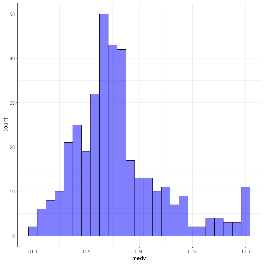

# test
ggplot(test_data, aes(medv)) + 
    geom_histogram(bins = 25, alpha = 0.5, fill = 'blue', color='black')  + 
    theme_bw()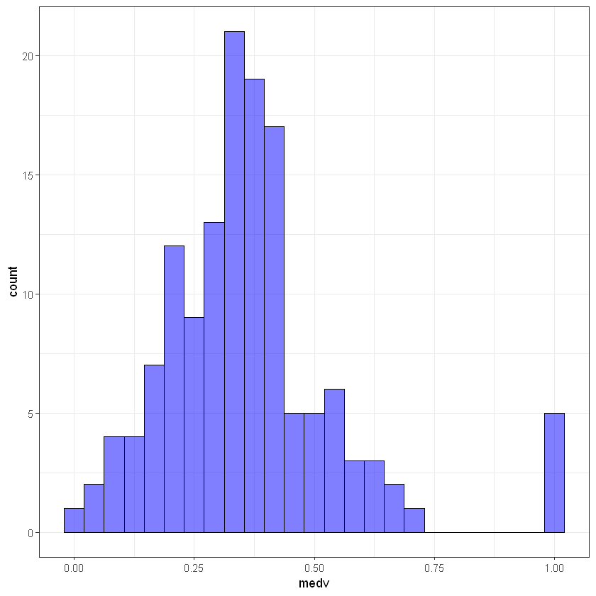

---

5.5 Baseline (Linear regression)

Для порівняння ефективності використання нейронних мереж скористаємося для початку лінійною регресією:

lm_model <- lm(medv ~ ., data = train_data)
summary(lm_model)

Call:
lm(formula = medv ~ ., data = train_data)

Residuals:
     Min       1Q   Median       3Q      Max 
-0.24556 -0.06405 -0.01292  0.04494  0.59898 

Coefficients:
            Estimate Std. Error t value Pr(>|t|)    
(Intercept)  0.49370    0.06281   7.860 4.70e-14 ***
crim        -0.14725    0.15139  -0.973 0.331410    
zn           0.08336    0.03588   2.323 0.020751 *  
indus        0.01499    0.04469   0.335 0.737541    
chas         0.01520    0.02281   0.667 0.505425    
nox         -0.18674    0.05028  -3.714 0.000237 ***
rm           0.48617    0.05571   8.727  < 2e-16 ***
age         -0.01314    0.03207  -0.410 0.682344    
dis         -0.36140    0.05961  -6.063 3.43e-09 ***
rad          0.14625    0.04369   3.347 0.000905 ***
tax         -0.14304    0.05333  -2.682 0.007655 ** 
ptratio     -0.21909    0.03199  -6.850 3.30e-11 ***
black        0.07181    0.02898   2.478 0.013692 *  
lstat       -0.41460    0.04909  -8.446 7.94e-16 ***
---
Signif. codes:  0 '***' 0.001 '**' 0.01 '*' 0.05 '.' 0.1 ' ' 1

Residual standard error: 0.1058 on 353 degrees of freedom
Multiple R-squared:  0.7566,    Adjusted R-squared:  0.7477 
F-statistic: 84.42 on 13 and 353 DF,  p-value: < 2.2e-16

Здійснимо прогноз тестових значень:

test_lm_predicted_scaled <- predict(lm_model, test_data)
head(test_lm_predicted_scaled)

1

0.56792431740972

5

0.523111676025518

20

0.295073007902457

29

0.32360237024043

30

0.355931690861336

35

0.195998476728651

test_lm_predicted <- sapply(X = test_lm_predicted_scaled, original = data$medv, FUN = revertData) %>% as.data.frame()
head(test_lm_predicted)

A data.frame: 6 × 1

	.
	<dbl>
1	30.55659
5	28.54003
20	18.27829
29	19.56211
30	21.01693
35	13.81993

Let’s check errors and R^2:

library(modelr)
# need for next comparison
linear_err <- data.frame(  
  R2_train = round(modelr::rsquare(lm_model, data = train_data), 4),
  R2_test = round(modelr::rsquare(lm_model, data = test_data), 4),
  MSE_test = round(modelr::mse(lm_model, data = test_data), 4),
  RMSE_test = round(modelr::rmse(lm_model, data = test_data), 4) 
)

rownames(linear_err) <- c("linear")
linear_err

A data.frame: 1 × 4

	R2_train	R2_test	MSE_test	RMSE_test
	<dbl>	<dbl>	<dbl>	<dbl>
linear	0.7566	0.6611	0.0117	0.1081

---

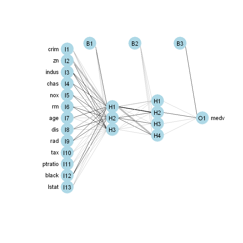
5.6 Побудова нейромережі за допомогою neuralnet

Підключаємо пакет neuralnet:

suppressMessages(library(neuralnet))

Attaching package: 'neuralnet'


The following object is masked from 'package:dplyr':

    compute

Для побудови моделі потрібно згенерувати формулу у форматі \(y ~ x_1 + x_2 + ... + x_n\)

n <- colnames(data)
n <- n[!n %in% "medv"]
formula <- as.formula(paste("medv ~", paste(n, collapse = " + ")))
formula

medv ~ crim + zn + indus + chas + nox + rm + age + dis + rad + 
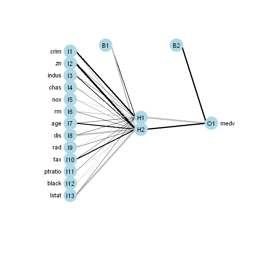
    tax + ptratio + black + lstat

Будуємо модель за допомогою фунуції neuralnet():

hidden = c(3,4) - перший прихований шар буде мати 3 нейрони, другий 4 linear.output - вихідний показник неперервне число. Не класифікація

nn_model <- neuralnet(formula = formula, data = train_data, hidden = c(3,4), linear.output = TRUE, rep = 1)

Візуалізуємо модель:

plot(nn_model)

train_data %>% head()

A data.frame: 6 × 14

	crim	zn	indus	chas	nox	rm	age	dis	rad	tax	ptratio	black	lstat	medv
	<dbl>	<dbl>	<dbl>	<dbl>	<dbl>	<dbl>	<dbl>	<dbl>	<dbl>	<dbl>	<dbl>	<dbl>	<dbl>	<dbl>
2	0.0002359225	0.000	0.24230205	0	0.1728395	0.5479977	0.7826982	0.3489620	0.04347826	0.10496183	0.5531915	1.0000000	0.20447020	0.3688889
3	0.0002356977	0.000	0.24230205	0	0.1728395	0.6943859	0.5993821	0.3489620	0.04347826	0.10496183	0.5531915	0.9897373	0.06346578	0.6600000
4	0.0002927957	0.000	0.06304985	0	0.1502058	0.6585553	0.4418126	0.4485446	0.08695652	0.06679389	0.6489362	0.9942761	0.03338852	0.6311111
6	0.0002644715	0.000	0.06304985	0	0.1502058	0.5497222	0.5746653	0.4485446	0.08695652	0.06679389	0.6489362	0.9929901	0.09602649	0.5266667
7	0.0009213230	0.125	0.27162757	0	0.2860082	0.4696302	0.6560247	0.4029226	0.17391304	0.23664122	0.2765957	0.9967220	0.29525386	0.3977778
8	0.0015536719	0.125	0.27162757	0	0.2860082	0.5002874	0.9598352	0.4383872	0.17391304	0.23664122	0.2765957	1.0000000	0.48068433	0.4911111

Також для візуалізація можна скористатися функцією plot.nnet(), опубілкованою на відкритому ресурсі одним із користувачів мережі Інтернет:

suppressMessages(library(devtools))

library(clusterGeneration)

suppressMessages(source_url('https://gist.githubusercontent.com/fawda123/7471137/raw/466c1474d0a505ff044412703516c34f1a4684a5/nnet_plot_update.r'))

suppressMessages(plot.nnet(nn_model))

Preview neural network matrix as text:

nn_model$result.matrix %>% head()

A matrix: 6 × 1 of type dbl

error	5.182582e-01
reached.threshold	9.322212e-03
steps	3.503000e+03
Intercept.to.1layhid1	5.249092e-01
crim.to.1layhid1	-2.880638e+00
zn.to.1layhid1	-9.485175e+01

Здійснимо прогноз для тестової вибірки та повернемо значення до базового виміру:

test_predicted_scaled <- compute(nn_model, test_data%>%select(-medv))

Convert $net.result to original form:

test_nn_predicted <- sapply(X = test_predicted_scaled$net.result, original = data$medv, FUN = revertData) %>% as.data.frame()
head(test_nn_predicted)

A data.frame: 6 × 1

	.
	<dbl>
1	28.74649
2	31.34932
3	18.86595
4	18.92882
5	19.89660
6	11.69719

Порівняємо похибки та \(R^2\) по лінійній регресії та першій нейронній мережі:

head(test_data)

A data.frame: 6 × 14

	crim	zn	indus	chas	nox	rm	age	dis	rad	tax	ptratio	black	lstat	medv
	<dbl>	<dbl>	<dbl>	<dbl>	<dbl>	<dbl>	<dbl>	<dbl>	<dbl>	<dbl>	<dbl>	<dbl>	<dbl>	<dbl>
1	0.0000000000	0.18	0.06781525	0	0.3148148	0.5775053	0.6416066	0.2692031	0.00000000	0.20801527	0.2872340	1.0000000	0.08967991	0.4222222
5	0.0007050701	0.00	0.06304985	0	0.1502058	0.6871048	0.5283213	0.4485446	0.08695652	0.06679389	0.6489362	1.0000000	0.09933775	0.6933333
20	0.0080867817	0.00	0.28152493	0	0.3148148	0.4150220	0.6858908	0.2425138	0.13043478	0.22900763	0.8936170	0.9849967	0.26352097	0.2933333
29	0.0086171860	0.00	0.28152493	0	0.3148148	0.5621767	0.9423275	0.3023670	0.13043478	0.22900763	0.8936170	0.9774068	0.30546358	0.2977778
30	0.0111962610	0.00	0.28152493	0	0.3148148	0.5964744	0.8692070	0.2827524	0.13043478	0.22900763	0.8936170	0.9579656	0.28283664	0.3555556
35	0.0180566727	0.00	0.28152493	0	0.3148148	0.4857252	0.9680742	0.2391765	0.13043478	0.22900763	0.8936170	0.6253215	0.51352097	0.1888889

suppressMessages(library(Metrics))

library(Metrics) # for rmse function
neuralnet_err <- data.frame(
  R2_train = round(cor(train_data$medv, nn_model$response[,"medv"])^2, 4),
  R2_test = round(cor(test_data$medv, test_predicted_scaled$net.result)^2, 4),
  MSE_test = round(mse(test_data$medv, test_predicted_scaled$net.result), 4),
  RMSE_test = round(rmse(test_data$medv, test_predicted_scaled$net.result), 4)  
)

rownames(neuralnet_err) <- "neuralnet"
linear_err |> bind_rows(neuralnet_err)

# Model is much better by all metrics but overfitted on train

A data.frame: 2 × 4

	R2_train	R2_test	MSE_test	RMSE_test
	<dbl>	<dbl>	<dbl>	<dbl>
linear	0.7566	0.6611	0.0117	0.1081
neuralnet	1.0000	0.7799	0.0077	0.0876

5.7 neuralnet + caret

suppressMessages(library(caret))

ctrl<- trainControl(method="cv", number=1, search="random")

suppressMessages(nn2_model <- train(formula, 
             data = train_data, 
             trControl = ctrl,
             metric = "RMSE",
             method = "neuralnet"))

head(nn2_model)

Warning message in cbind(intercept = 1, as.matrix(data[, model.list$variables])):
"number of rows of result is not a multiple of vector length (arg 1)"
Warning message in cbind(1, act.temp):
"number of rows of result is not a multiple of vector length (arg 1)"
Warning message in cbind(1, act.temp):
"number of rows of result is not a multiple of vector length (arg 1)"
Warning message in cbind(1, act.temp):
"number of rows of result is not a multiple of vector length (arg 1)"
Warning message in cbind(intercept = 1, as.matrix(data[, model.list$variables])):
"number of rows of result is not a multiple of vector length (arg 1)"
Warning message in cbind(1, act.temp):
"number of rows of result is not a multiple of vector length (arg 1)"
Warning message in cbind(1, act.temp):
"number of rows of result is not a multiple of vector length (arg 1)"
Warning message in cbind(1, act.temp):
"number of rows of result is not a multiple of vector length (arg 1)"
Warning message in cbind(intercept = 1, as.matrix(data[, model.list$variables])):
"number of rows of result is not a multiple of vector length (arg 1)"
Warning message in cbind(1, act.temp):
"number of rows of result is not a multiple of vector length (arg 1)"
Warning message in cbind(1, act.temp):
"number of rows of result is not a multiple of vector length (arg 1)"
Warning message in cbind(1, act.temp):
"number of rows of result is not a multiple of vector length (arg 1)"

$method

'neuralnet'

$modelInfo

$label

'Neural Network'

$library

'neuralnet'

$loop

NULL

$type

'Regression'

$parameters

A data.frame: 3 × 3

parameter	class	label
<chr>	<chr>	<chr>
layer1	numeric	#Hidden Units in Layer 1
layer2	numeric	#Hidden Units in Layer 2
layer3	numeric	#Hidden Units in Layer 3

$grid

function (x, y, len = NULL, search = "grid") 
{
    if (search == "grid") {
        out <- expand.grid(layer1 = ((1:len) * 2) - 1, layer2 = 0, 
            layer3 = 0)
    }
    else {
        out <- data.frame(layer1 = sample(2:20, replace = TRUE, 
            size = len), layer2 = sample(c(0, 2:20), replace = TRUE, 
            size = len), layer3 = sample(c(0, 2:20), replace = TRUE, 
            size = len))
    }
    out
}

$fit

function (x, y, wts, param, lev, last, classProbs, ...) 
{
    colNames <- colnames(x)
    dat <- if (is.data.frame(x)) 
        x
    else as.data.frame(x, stringsAsFactors = TRUE)
    dat$.outcome <- y
    form <- as.formula(paste(".outcome ~", paste(colNames, collapse = "+")))
    if (param$layer1 == 0) 
        stop("the first layer must have at least one hidden unit")
    if (param$layer2 == 0 & param$layer2 > 0) 
        stop("the second layer must have at least one hidden unit if a third layer is specified")
    nodes <- c(param$layer1)
    if (param$layer2 > 0) {
        nodes <- c(nodes, param$layer2)
        if (param$layer3 > 0) 
            nodes <- c(nodes, param$layer3)
    }
    neuralnet::neuralnet(form, data = dat, hidden = nodes, ...)
}

$predict

function (modelFit, newdata, submodels = NULL) 
{
    newdata <- newdata[, modelFit$model.list$variables, drop = FALSE]
    neuralnet::compute(modelFit, covariate = newdata)$net.result[, 
        1]
}

$prob

NULL

$tags

'Neural Network'

$sort

function (x) 
x[order(x$layer1, x$layer2, x$layer3), ]

$modelType

'Regression'

$results

A data.frame: 3 × 9

	layer1	layer2	layer3	RMSE	Rsquared	MAE	RMSESD	RsquaredSD	MAESD
	<int>	<dbl>	<dbl>	<dbl>	<dbl>	<dbl>	<dbl>	<dbl>	<dbl>
1	4	2	15	4.317601	0.0009609744	4.312419	NA	NA	NA
2	11	7	10	2.110006	0.1077528131	2.098059	NA	NA	NA
3	15	6	7	2.774424	0.0840212438	2.766978	NA	NA	NA

$pred

NULL

$bestTune

A data.frame: 1 × 3

	layer1	layer2	layer3
	<int>	<dbl>	<dbl>
2	11	7	10

test_predicted_scaled <- predict(nn2_model, test_data%>%select(-medv))
head(test_predicted_scaled)
train_predicted_scaled <- predict(nn2_model, train_data%>%select(-medv))
head(train_predicted_scaled)

1

0.487043261409714

5

0.621601182176565

20

0.296898662765632

29

0.311093959706198

30

0.358306907905892

35

0.207608926759425

2

0.404953900784053

3

0.631590265523993

4

0.616779701435411

6

0.485288600524427

7

0.344873486827333

8

0.321661962365258

test_nn2_predicted <- sapply(X = test_predicted_scaled, original = data$medv, FUN = revertData) %>% as.data.frame()
head(test_nn2_predicted)

A data.frame: 6 × 1

	.
	<dbl>
1	26.91695
5	32.97205
20	18.36044
29	18.99923
30	21.12381
35	14.34240

neuralnet2_err <- data.frame(
  R2_train = round(cor(train_data$medv, train_predicted_scaled)^2, 4),
  R2_test = round(cor(test_data$medv, test_predicted_scaled)^2, 4),
  MSE_test = round(mse(test_data$medv, test_predicted_scaled), 4),
  RMSE_test = round(rmse(test_data$medv, test_predicted_scaled), 4)  
)

rownames(neuralnet2_err) <- "neuralnet_caret"
linear_err |> bind_rows(neuralnet_err) |> bind_rows(neuralnet2_err)

A data.frame: 3 × 4

	R2_train	R2_test	MSE_test	RMSE_test
	<dbl>	<dbl>	<dbl>	<dbl>
linear	0.7566	0.6611	0.0117	0.1081
neuralnet	1.0000	0.7799	0.0077	0.0876
neuralnet_caret	0.9767	0.8251	0.0063	0.0793

---

5.8 Neural network with nnet

Підключаємо пакет nnet для побудови нейромережі із 2-ма прихованими шарами, для прикладу.

library(nnet)

Будуємо модель на основі формули створеної для попередньої моделі:

• size - кількість нейронів у прихованому шарі

nnet_model <- nnet(formula, data = train_data, size = 2, maxit = 100)
# Не забудьте поекспериментувати зі зміною кількості вузлів

Your code contains a unicode char which cannot be displayed in your
current locale and R will silently convert it to an escaped form when the
R kernel executes this code. This can lead to subtle errors if you use
such chars to do comparisons. For more information, please see
https://github.com/IRkernel/repr/wiki/Problems-with-unicode-on-windows

# weights:  31
initial  value 17.172411 
iter  10 value 3.798860
iter  20 value 2.477108
iter  30 value 2.048115
iter  40 value 1.889895
iter  50 value 1.692867
iter  60 value 1.452958
iter  70 value 1.436145
iter  80 value 1.420405
iter  90 value 1.398269
iter 100 value 1.390185
final  value 1.390185 
stopped after 100 iterations

summary(nnet_model)

a 13-2-1 network with 31 weights
options were -
  b->h1  i1->h1  i2->h1  i3->h1  i4->h1  i5->h1  i6->h1  i7->h1  i8->h1  i9->h1 
   3.21   11.13    0.13    0.14   -0.03   -0.12   -2.78    0.39    0.45   -0.59 
i10->h1 i11->h1 i12->h1 i13->h1 
   0.46    0.36   -0.51    0.46 
  b->h2  i1->h2  i2->h2  i3->h2  i4->h2  i5->h2  i6->h2  i7->h2  i8->h2  i9->h2 
 -10.30   -2.70   14.50    3.19    0.10   -2.68    1.65    7.43  -14.01    0.98 
i10->h2 i11->h2 i12->h2 i13->h2 
   8.10   -2.17   -1.77  -14.95 
  b->o  h1->o  h2->o 
 10.26 -12.12   8.44 

Візуалізуємо модель:

plot.nnet(nnet_model)

Здійснимо прогноз для тестової вибірки та повернемо значення до базового виміру:

test_predicted_scaled <- predict(nnet_model, test_data)
head(test_predicted_scaled)
test_nnet_predicted <- sapply(X = test_predicted_scaled, original = data$medv, FUN = revertData) %>% as.data.frame()

A matrix: 6 × 1 of type dbl

1	0.5002897
5	0.6030015
20	0.2798733
29	0.3302058
30	0.3558518
35	0.2345779

nnet_model

a 13-2-1 network with 31 weights
inputs: crim zn indus chas nox rm age dis rad tax ptratio black lstat 
output(s): medv 
options were -

Порівняємо похибки по лінійній регресії та нейронних мереж:

nnet_err <- data.frame(
  R2_train = round(cor(train_data$medv, predict(nnet_model, new=train_data))^2, 4),
  R2_test = round(cor(test_data$medv, test_predicted_scaled)^2, 4),
  MSE_test = round(mse(test_data$medv, test_predicted_scaled), 4),
  RMSE_test = round(rmse(test_data$medv, test_predicted_scaled), 4)  
)

rownames(nnet_err) <- "nnet"
linear_err |> bind_rows(neuralnet_err) |> bind_rows(neuralnet2_err) |> bind_rows(nnet_err)

# neuralnet wins! but remember it has more layers

A data.frame: 4 × 4

	R2_train	R2_test	MSE_test	RMSE_test
	<dbl>	<dbl>	<dbl>	<dbl>
linear	0.7566	0.6611	0.0117	0.1081
neuralnet	1.0000	0.7799	0.0077	0.0876
neuralnet_caret	0.9767	0.8251	0.0063	0.0793
nnet	0.9148	0.7276	0.0103	0.1013

---

5.9 Final models compare

Побудуємо графік розподілу пронозованих значень показників по усх моделях:

head(test_lm_predicted)
head(test_nn_predicted)
head(test_nnet_predicted)

A data.frame: 6 × 1

	.
	<dbl>
1	30.55659
5	28.54003
20	18.27829
29	19.56211
30	21.01693
35	13.81993

A data.frame: 6 × 1

	.
	<dbl>
1	28.74649
2	31.34932
3	18.86595
4	18.92882
5	19.89660
6	11.69719

A data.frame: 6 × 1

	.
	<dbl>
1	27.51304
2	32.13507
3	17.59430
4	19.85926
5	21.01333
6	15.55600

test_medv <- subset(data, !split) |> select(medv) |> unlist()
head(test_medv)

medv1

24

medv2

36.2

medv3

18.2

medv4

18.4

medv5

21

medv6

13.5

head(test_data)

A data.frame: 6 × 14

	crim	zn	indus	chas	nox	rm	age	dis	rad	tax	ptratio	black	lstat	medv
	<dbl>	<dbl>	<dbl>	<dbl>	<dbl>	<dbl>	<dbl>	<dbl>	<dbl>	<dbl>	<dbl>	<dbl>	<dbl>	<dbl>
1	0.0000000000	0.18	0.06781525	0	0.3148148	0.5775053	0.6416066	0.2692031	0.00000000	0.20801527	0.2872340	1.0000000	0.08967991	0.4222222
5	0.0007050701	0.00	0.06304985	0	0.1502058	0.6871048	0.5283213	0.4485446	0.08695652	0.06679389	0.6489362	1.0000000	0.09933775	0.6933333
20	0.0080867817	0.00	0.28152493	0	0.3148148	0.4150220	0.6858908	0.2425138	0.13043478	0.22900763	0.8936170	0.9849967	0.26352097	0.2933333
29	0.0086171860	0.00	0.28152493	0	0.3148148	0.5621767	0.9423275	0.3023670	0.13043478	0.22900763	0.8936170	0.9774068	0.30546358	0.2977778
30	0.0111962610	0.00	0.28152493	0	0.3148148	0.5964744	0.8692070	0.2827524	0.13043478	0.22900763	0.8936170	0.9579656	0.28283664	0.3555556
35	0.0180566727	0.00	0.28152493	0	0.3148148	0.4857252	0.9680742	0.2391765	0.13043478	0.22900763	0.8936170	0.6253215	0.51352097	0.1888889

#Однакові межі для усіх графіків по Y
plot_ylim <- c(5,40)

par(mfrow=c(1,3)) # три стовпці, 1 рядок
# pch  - тип точки для графіку
plot(test_medv, test_lm_predicted[,1], col='black', ylim=plot_ylim, main='Real vs predicted LM', pch=25, cex=0.7)
abline(0,1,lwd=2)
legend('bottomright',legend='LM',pch=25,col='black', bty='n')

plot(test_medv,test_nn_predicted[,1], col='red', ylim=plot_ylim, main='Real vs predicted NN',pch=18,cex=0.7)
abline(0,1,lwd=2)
legend('bottomright',legend='NN',pch=18,col='red', bty='n')

plot(test_medv,test_nnet_predicted[,1], col='blue', ylim=plot_ylim, main='Real vs predicted NNET',pch=18,cex=0.7)
abline(0,1,lwd=2)

legend('bottomright',legend='NNET',pch=18, col='black', bty='n')

Your code contains a unicode char which cannot be displayed in your
current locale and R will silently convert it to an escaped form when the
R kernel executes this code. This can lead to subtle errors if you use
such chars to do comparisons. For more information, please see
https://github.com/IRkernel/repr/wiki/Problems-with-unicode-on-windows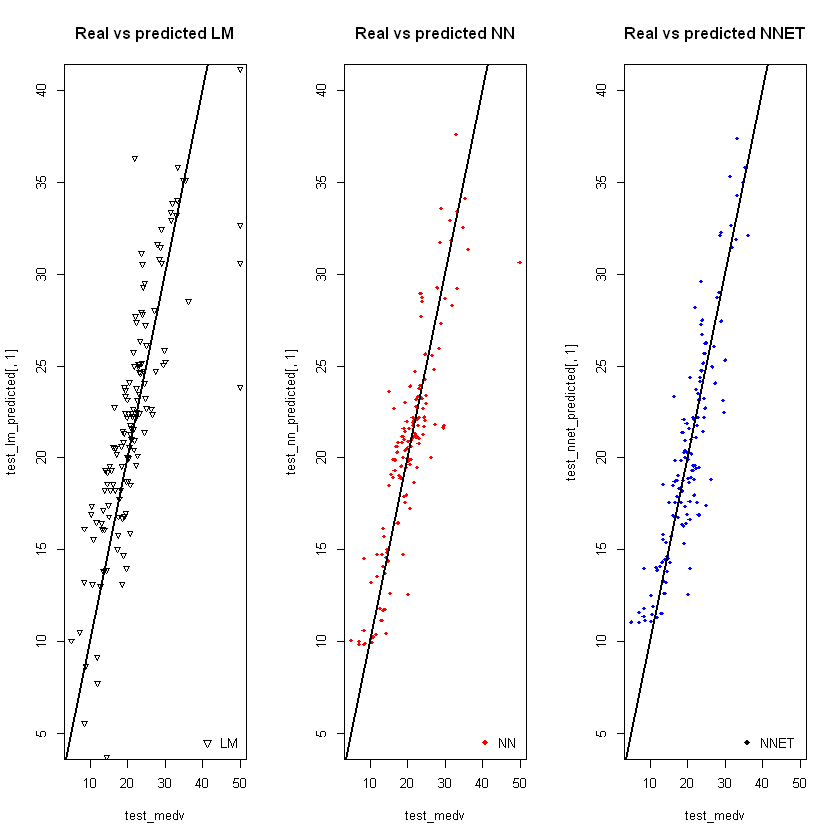

Combine all to one chart:

par(mfrow=c(1,1))

plot(test_medv,test_lm_predicted[,1],col='black',main='Real vs predicted NN + LM',pch=25,cex=0.7)
points(test_medv,test_nn_predicted[,1],col='red',pch=19,cex=0.7)
points(test_medv,test_nnet_predicted[,1],col='blue',pch=18,cex=0.7)
abline(0,1,lwd=2)
legend('bottomright',legend=c('lm','neuralnet','nnet'),pch=c(25,19,18),col=c('black', 'red','blue'))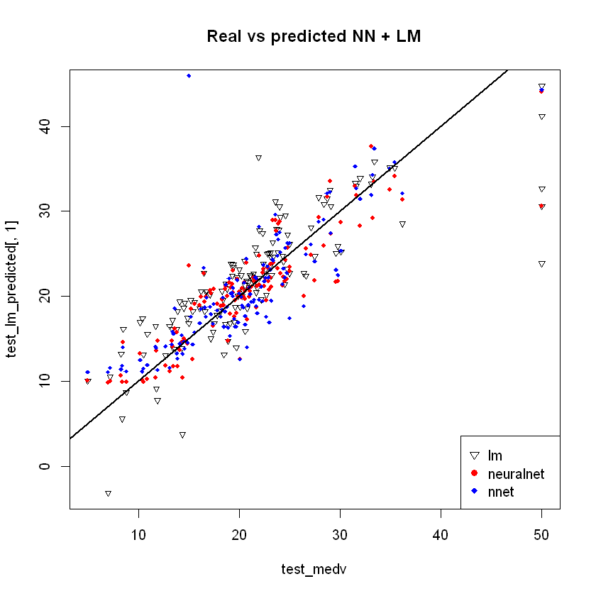

---

5.10 Валідація моделі на різних розмірах вибірки

suppressMessages(library(boot))
suppressMessages(library(plyr))
suppressMessages(library(DMwR))

set.seed(2023)
errors <- data.frame(TrainSize = c(1:90), RMSE1 = c(0), RMSE2 = c(0))

for(i in 1:10) {

    for(j in 1:90){
  
      split <- c(1:(nrow(scaled_data)*j/100))
  
      train_data <- scaled_data[split,]
      test_data <- scaled_data[-split,]
  
      nnet_model <- nnet(formula, data = train_data,  size = 3, maxit = 100, trace = F)
  
      nnet_predicted_prob_scaled <- predict(nnet_model, test_data)
      nnet_predicted <- nnet_predicted_prob_scaled * (max(data$medv) - min(data$medv)) + min(data$medv)
  
      errors_list <- regr.eval(test_data$medv, nnet_predicted)
  
      errors[errors$TrainSize == j, ]$RMSE1 <- errors[errors$TrainSize == j, ]$RMSE1 + errors_list[3]
    }
}

Attaching package: 'boot'


The following object is masked from 'package:lattice':

    melanoma


------------------------------------------------------------------------------

You have loaded plyr after dplyr - this is likely to cause problems.
If you need functions from both plyr and dplyr, please load plyr first, then dplyr:
library(plyr); library(dplyr)

------------------------------------------------------------------------------


Attaching package: 'plyr'


The following objects are masked from 'package:reshape':

    rename, round_any


The following objects are masked from 'package:dplyr':

    arrange, count, desc, failwith, id, mutate, rename, summarise,
    summarize


Loading required package: grid

Registered S3 method overwritten by 'quantmod':
  method            from
  as.zoo.data.frame zoo 


Attaching package: 'DMwR'


The following object is masked from 'package:plyr':

    join


The following object is masked from 'package:modelr':

    bootstrap

errors$RMSE1 <- errors$RMSE1/10
plot (x = errors$TrainSize, 
      y = errors$RMSE1, 
      ylim = c(min(errors$RMSE1), 
               max(errors$RMSE1)), 
      type = "l", 
      xlab = "length of training set", 
      ylab = "mean RMSE", 
      main = "Variation of RMSE with length of training set")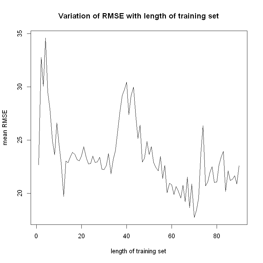

for(i in 1:10) {
  
  for(j in 1:90){
    
    split <- sample.split(scaled_data$medv, SplitRatio = j/100)
    
    train_data <- subset(scaled_data, split == TRUE)
    test_data <- subset(scaled_data, split == FALSE)
    
    nnet_model <- nnet(formula, data = train_data,  size = 3, maxit = 100, trace = F)
    
    nnet_predicted_prob_scaled <- predict(nnet_model, test_data)
    nnet_predicted <- nnet_predicted_prob_scaled * (max(data$medv) - min(data$medv)) + min(data$medv)
      
    errors_list <- regr.eval(test_data$medv, nnet_predicted)
    
    errors[errors$TrainSize == j, ]$RMSE2 <- errors[errors$TrainSize == j, ]$RMSE2 + errors_list[3]
  }
}

errors$RMSE2 <- errors$RMSE2/10
plot (x = errors$TrainSize, 
      y = errors$RMSE2, 
      ylim = c(min(errors$RMSE2), 
               max(errors$RMSE2)), 
      type = "l", 
      xlab = "length of training set", 
      ylab = "mean RMSE", 
      main = "Variation of RMSE with length of training set")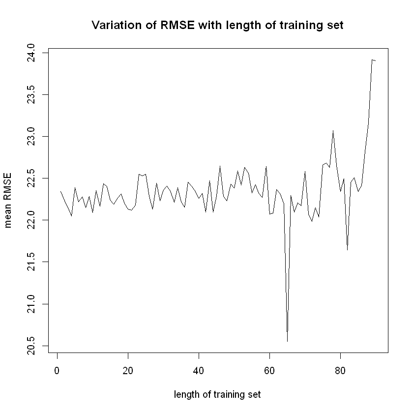

head(errors)

A data.frame: 6 × 3

	TrainSize	RMSE1	RMSE2
	<int>	<dbl>	<dbl>
1	1	22.65845	22.34442
2	2	32.76667	22.23155
3	3	30.06977	22.14714
4	4	34.59365	22.05084
5	5	29.49516	22.39201
6	6	27.93207	22.22010

---

require(caret)

folds <- createFolds(scaled_data$medv, k = 10, list = TRUE, returnTrain = FALSE)
errors2 <- data.frame(FoldExcluded = c(1:10), RMSE = c(0))

folds

$Fold01

1. 16
2. 20
3. 21
4. 39
5. 46
6. 47
7. 48
8. 56
9. 69
10. 91
11. 120
12. 127
13. 132
14. 143
15. 151
16. 186
17. 187
18. 191
19. 196
20. 227
21. 231
22. 236
23. 239
24. 252
25. 258
26. 259
27. 279
28. 280
29. 289
30. 314
31. 320
32. 335
33. 337
34. 350
35. 352
36. 360
37. 372
38. 373
39. 380
40. 385
41. 392
42. 409
43. 415
44. 419
45. 420
46. 431
47. 439
48. 445
49. 452
50. 468
51. 484
52. 486

$Fold02

1. 5
2. 15
3. 22
4. 23
5. 33
6. 34
7. 35
8. 52
9. 79
10. 80
11. 88
12. 97
13. 98
14. 126
15. 130
16. 135
17. 160
18. 168
19. 184
20. 205
21. 230
22. 243
23. 253
24. 261
25. 263
26. 267
27. 270
28. 273
29. 304
30. 313
31. 319
32. 354
33. 366
34. 387
35. 389
36. 411
37. 422
38. 423
39. 440
40. 451
41. 454
42. 463
43. 467
44. 478
45. 480
46. 482
47. 483
48. 498
49. 504

$Fold03

1. 4
2. 17
3. 26
4. 38
5. 53
6. 70
7. 71
8. 82
9. 86
10. 100
11. 104
12. 128
13. 133
14. 134
15. 141
16. 147
17. 201
18. 208
19. 209
20. 212
21. 214
22. 217
23. 224
24. 246
25. 269
26. 274
27. 305
28. 325
29. 326
30. 332
31. 341
32. 348
33. 353
34. 355
35. 356
36. 362
37. 365
38. 369
39. 370
40. 377
41. 382
42. 390
43. 400
44. 404
45. 407
46. 408
47. 417
48. 418
49. 470
50. 495
51. 501

$Fold04

1. 3
2. 9
3. 28
4. 68
5. 72
6. 77
7. 87
8. 89
9. 93
10. 95
11. 131
12. 139
13. 140
14. 144
15. 163
16. 195
17. 197
18. 204
19. 213
20. 229
21. 233
22. 248
23. 254
24. 284
25. 290
26. 291
27. 299
28. 300
29. 301
30. 303
31. 316
32. 317
33. 318
34. 327
35. 329
36. 333
37. 339
38. 342
39. 346
40. 349
41. 351
42. 363
43. 391
44. 393
45. 399
46. 406
47. 426
48. 441
49. 450
50. 472
51. 473
52. 476

$Fold05

1. 55
2. 76
3. 85
4. 94
5. 113
6. 117
7. 118
8. 125
9. 142
10. 156
11. 157
12. 159
13. 167
14. 170
15. 172
16. 179
17. 189
18. 190
19. 192
20. 194
21. 203
22. 221
23. 240
24. 262
25. 272
26. 285
27. 286
28. 310
29. 324
30. 330
31. 338
32. 344
33. 358
34. 368
35. 371
36. 388
37. 414
38. 425
39. 427
40. 429
41. 434
42. 449
43. 459
44. 475
45. 493
46. 497
47. 500
48. 503
49. 505

$Fold06

1. 11
2. 13
3. 14
4. 41
5. 42
6. 45
7. 57
8. 62
9. 63
10. 106
11. 108
12. 114
13. 116
14. 119
15. 121
16. 136
17. 137
18. 153
19. 171
20. 176
21. 177
22. 199
23. 202
24. 207
25. 215
26. 223
27. 226
28. 234
29. 235
30. 244
31. 257
32. 281
33. 282
34. 288
35. 292
36. 302
37. 307
38. 312
39. 334
40. 336
41. 379
42. 395
43. 413
44. 428
45. 433
46. 435
47. 444
48. 446
49. 453
50. 456
51. 485

$Fold07

1. 1
2. 7
3. 10
4. 12
5. 27
6. 30
7. 40
8. 58
9. 60
10. 73
11. 74
12. 78
13. 81
14. 83
15. 92
16. 96
17. 152
18. 154
19. 158
20. 162
21. 169
22. 206
23. 210
24. 216
25. 218
26. 237
27. 242
28. 245
29. 249
30. 260
31. 266
32. 276
33. 293
34. 295
35. 311
36. 321
37. 345
38. 347
39. 357
40. 378
41. 383
42. 386
43. 405
44. 424
45. 438
46. 447
47. 448
48. 455
49. 457
50. 458
51. 460

$Fold08

1. 8
2. 24
3. 29
4. 32
5. 43
6. 102
7. 105
8. 110
9. 111
10. 112
11. 123
12. 124
13. 146
14. 149
15. 165
16. 166
17. 173
18. 175
19. 181
20. 183
21. 200
22. 220
23. 222
24. 225
25. 247
26. 251
27. 264
28. 271
29. 278
30. 283
31. 287
32. 296
33. 297
34. 331
35. 340
36. 359
37. 364
38. 376
39. 394
40. 398
41. 432
42. 443
43. 461
44. 469
45. 479
46. 488
47. 490
48. 491
49. 496
50. 506

$Fold09

1. 6
2. 18
3. 19
4. 25
5. 36
6. 50
7. 54
8. 59
9. 61
10. 66
11. 90
12. 99
13. 103
14. 107
15. 109
16. 155
17. 161
18. 164
19. 174
20. 178
21. 180
22. 182
23. 198
24. 211
25. 219
26. 250
27. 265
28. 275
29. 306
30. 328
31. 361
32. 367
33. 375
34. 381
35. 384
36. 396
37. 397
38. 402
39. 403
40. 412
41. 416
42. 437
43. 442
44. 464
45. 465
46. 466
47. 471
48. 477
49. 481
50. 502

$Fold10

1. 2
2. 31
3. 37
4. 44
5. 49
6. 51
7. 64
8. 65
9. 67
10. 75
11. 84
12. 101
13. 115
14. 122
15. 129
16. 138
17. 145
18. 148
19. 150
20. 185
21. 188
22. 193
23. 228
24. 232
25. 238
26. 241
27. 255
28. 256
29. 268
30. 277
31. 294
32. 298
33. 308
34. 309
35. 315
36. 322
37. 323
38. 343
39. 374
40. 401
41. 410
42. 421
43. 430
44. 436
45. 462
46. 474
47. 487
48. 489
49. 492
50. 494
51. 499

for(i in 1:10) {
  
  for(j in 1:10){    
    train_data <- scaled_data[-folds[[j]], ]
    test_data <- scaled_data[folds[[j]], ]
    
    nnet_model <- nnet(formula, data = train_data, trace = F,  size = 3, maxit = 100)
    
    nnet_predicted_prob_scaled <- predict(nnet_model, test_data)
    nnet_predicted <- nnet_predicted_prob_scaled * (max(data$medv) - min(data$medv)) + min(data$medv)
    errors_list <- regr.eval(test_data$medv, nnet_predicted)
    errors2[errors2$FoldExcluded == j, ]$RMSE <- errors2[errors2$FoldExcluded == j, ]$RMSE + errors_list[3]
  }
}

errors2$RMSE <- errors2$RMSE/10
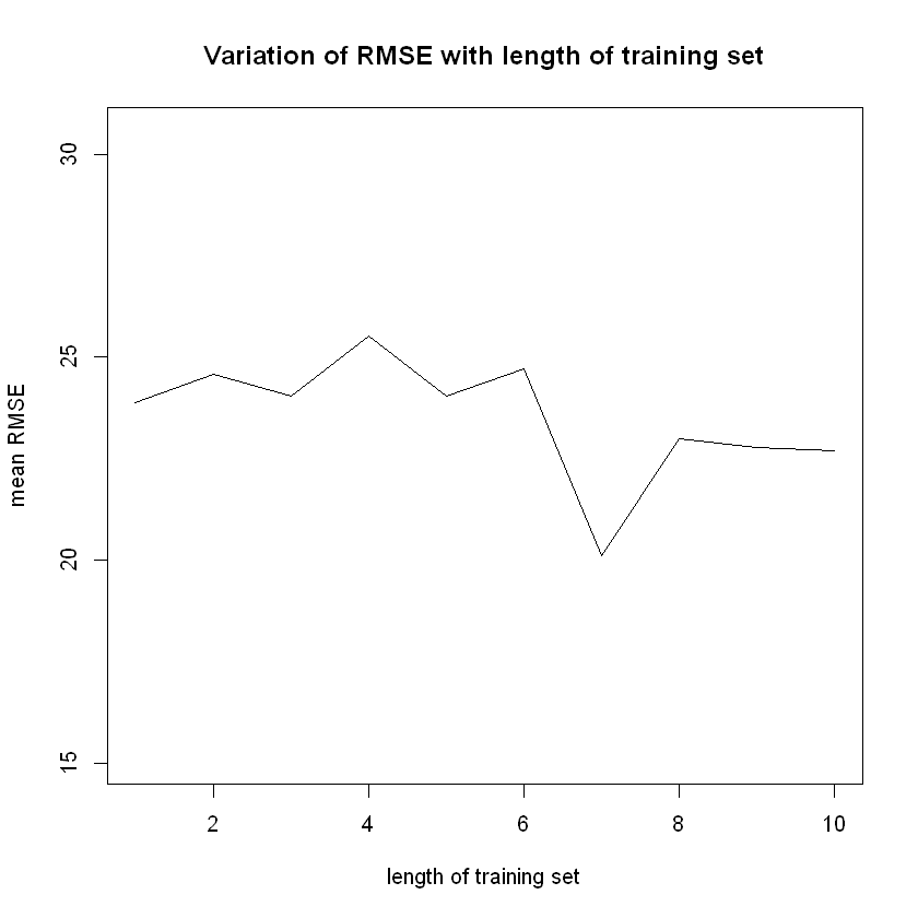
plot (x = errors2$FoldExcluded, y = errors2$RMSE, 
      ylim = c(min(errors2$RMSE)-5, 
               max(errors2$RMSE)+5), 
      type = "l", 
      xlab = "length of training set", 
      ylab = "mean RMSE", 
      main = "Variation of RMSE with length of training set")
head(errors2)

A data.frame: 6 × 2

	FoldExcluded	RMSE
	<int>	<dbl>
1	1	23.88887
2	2	24.57703
3	3	24.03482
4	4	25.52928
5	5	24.05225
6	6	24.70978

---

6 References

1. Harrison, D. and Rubinfeld, D.L. (1978) Hedonic prices and the demand for clean air. J. Environ. Economics and Management 5, 81–102.

2. Belsley D.A., Kuh, E. and Welsch, R.E. (1980) Regression Diagnostics. Identifying Influential Data and Sources of Collinearity. New York: Wiley.