7  Дерева рішень. Класифікація. Депозити

Курс: “Математичне моделювання в R”

---

У даній частині навчального процесу потрібно побудувати математичні моделі класифікації клієнтів на основі алгоритму дерева рішень та перевірити їх на тестовій вибірці.

# install.packages("C50")
# install.packages("xgboost")
# install.packages("scorecard")
# install.packages("lightgbm")
# install.packages("Matrix") 
# install.packages("scorecard") 

7.1 Dataset description

Abstract

The data is related with direct marketing campaigns (phone calls) of a Portuguese banking institution. The classification goal is to predict if the client will subscribe a term deposit (variable y).

Data Set Information:

The data is related with direct marketing campaigns of a Portuguese banking institution. The marketing campaigns were based on phone calls. Often, more than one contact to the same client was required, in order to access if the product (bank term deposit) would be (‘yes’) or not (‘no’) subscribed.

There are four datasets: 1. bank-additional-full.csv with all examples (41188) and 20 inputs, ordered by date (from May 2008 to November 2010), very close to the data analyzed in [Moro et al., 2014] 2. bank-additional.csv with 10% of the examples (4119), randomly selected from 1), and 20 inputs. 3. bank-full.csv with all examples and 17 inputs, ordered by date (older version of this dataset with less inputs). 4. bank.csv with 10% of the examples and 17 inputs, randomly selected from 3 (older version of this dataset with less inputs).

The smallest datasets are provided to test more computationally demanding machine learning algorithms (e.g., SVM).

The classification goal is to predict if the client will subscribe (yes/no) a term deposit (variable y).

Attribute Information

Input variables: bank client data:

No	Title	Description	Data Type	Values
1	age		numeric
2	job	type of job	categorical	‘admin.’, ‘blue-collar’, ‘entrepreneur’, ‘housemaid’, ‘management’, ‘retired’, ‘self-employed’, ‘services’, ‘student’, ‘technician’, ‘unemployed’, ‘unknown’
3	marital	marital status	categorical	‘divorced’,‘married’,‘single’,‘unknown’; note: ‘divorced’ means divorced or widowed
4	education		categorical	‘basic.4y’,‘basic.6y’,‘basic.9y’,‘high.school’,‘illiterate’,‘professional.course’,‘university.degree’,‘unknown’
5	default	has credit in default?	categorical	‘no’,‘yes’,‘unknown’
6	housing	has housing loan?	categorical	‘no’,‘yes’,‘unknown’
7	loan	has personal loan?	categorical	‘no’,‘yes’,‘unknown’

Input variables: related with the last contact of the current campaign:

No	Title	Description	Data Type	Values
8	contact	contact communication type	categorical	‘cellular’,‘telephone’
9	month	last contact month of year	categorical	‘jan’, ‘feb’, ‘mar’, …, ‘nov’, ‘dec’
10	day_of_week	last contact day of the week	categorical	‘mon’,‘tue’,‘wed’,‘thu’,‘fri’
11	duration	last contact duration, in seconds	numeric

duration - Important note: this attribute highly affects the output target (e.g., if duration=0 then y=‘no’). Yet, the duration is not known before a call is performed. Also, after the end of the call y is obviously known. Thus, this input should only be included for benchmark purposes and should be discarded if the intention is to have a realistic predictive model.

Input variables: other attributes:

No	Title	Description	Data Type	Values
12	campaign	number of contacts performed during this campaign and for this client	numeric	includes last contact
13	pdays	number of days that passed by after the client was last contacted from a previous campaign	numeric	999 mean client was not previously contacted
14	previous	number of contacts performed before this campaign and for this client	numeric
15	poutcome	outcome of the previous marketing campaign	categorical	‘failure’,‘nonexistent’,‘success’

Input variables: social and economic context attributes

No	Title	Description	Data Type	Values
16	emp.var.rate	employment variation rate - quarterly indicator	numeric
17	cons.price.idx	consumer price index - monthly indicator	numeric
18	cons.conf.idx	consumer confidence index - monthly indicator		numeric
19	euribor3m	euribor 3 month rate - daily indicator	numeric
20	nr.employed	number of employees - quarterly indicator	numeric

Output variable (desired target):

No	Title	Description	Data Type	Values
21	y	has the client subscribed a term deposit?	binary	‘yes’,‘no’

Source: https://archive.ics.uci.edu/ml/datasets/bank+marketing

---

7.2 Data load and preview

Для початку завантажимо дані у змінну data:

data <- read.csv("https://raw.githubusercontent.com/kleban/r-course-eng/main/data/banking.csv", 
                 na.strings = c("", " ", "NA", "NULL"), # fix missing as NA if present
                 stringsAsFactors = TRUE) # set strings as factor, we need this for some algorithms
#use + unknown with na.strings if you want to play with missing
#data <- read.csv("data/banking.csv", na.strings = c("", " ", "NA", "NULL", "unknown"))

Переглянемо структуру вибірки даних з str():

str(data)

'data.frame':   11162 obs. of  17 variables:
 $ age      : int  59 56 41 55 54 42 56 60 37 28 ...
 $ job      : Factor w/ 12 levels "admin.","blue-collar",..: 1 1 10 8 1 5 5 6 10 8 ...
 $ marital  : Factor w/ 3 levels "divorced","married",..: 2 2 2 2 2 3 2 1 2 3 ...
 $ education: Factor w/ 4 levels "primary","secondary",..: 2 2 2 2 3 3 3 2 2 2 ...
 $ default  : Factor w/ 2 levels "no","yes": 1 1 1 1 1 1 1 1 1 1 ...
 $ balance  : int  2343 45 1270 2476 184 0 830 545 1 5090 ...
 $ housing  : Factor w/ 2 levels "no","yes": 2 1 2 2 1 2 2 2 2 2 ...
 $ loan     : Factor w/ 2 levels "no","yes": 1 1 1 1 1 2 2 1 1 1 ...
 $ contact  : Factor w/ 3 levels "cellular","telephone",..: 3 3 3 3 3 3 3 3 3 3 ...
 $ day      : int  5 5 5 5 5 5 6 6 6 6 ...
 $ month    : Factor w/ 12 levels "apr","aug","dec",..: 9 9 9 9 9 9 9 9 9 9 ...
 $ duration : int  1042 1467 1389 579 673 562 1201 1030 608 1297 ...
 $ campaign : int  1 1 1 1 2 2 1 1 1 3 ...
 $ pdays    : int  -1 -1 -1 -1 -1 -1 -1 -1 -1 -1 ...
 $ previous : int  0 0 0 0 0 0 0 0 0 0 ...
 $ poutcome : Factor w/ 4 levels "failure","other",..: 4 4 4 4 4 4 4 4 4 4 ...
 $ deposit  : Factor w/ 2 levels "no","yes": 2 2 2 2 2 2 2 2 2 2 ...

Переглянемо вигляд перших рядків даних з head():

head(data)

A data.frame: 6 × 17

	age	job	marital	education	default	balance	housing	loan	contact	day	month	duration	campaign	pdays	previous	poutcome	deposit
	<int>	<fct>	<fct>	<fct>	<fct>	<int>	<fct>	<fct>	<fct>	<int>	<fct>	<int>	<int>	<int>	<int>	<fct>	<fct>
1	59	admin.	married	secondary	no	2343	yes	no	unknown	5	may	1042	1	-1	0	unknown	yes
2	56	admin.	married	secondary	no	45	no	no	unknown	5	may	1467	1	-1	0	unknown	yes
3	41	technician	married	secondary	no	1270	yes	no	unknown	5	may	1389	1	-1	0	unknown	yes
4	55	services	married	secondary	no	2476	yes	no	unknown	5	may	579	1	-1	0	unknown	yes
5	54	admin.	married	tertiary	no	184	no	no	unknown	5	may	673	2	-1	0	unknown	yes
6	42	management	single	tertiary	no	0	yes	yes	unknown	5	may	562	2	-1	0	unknown	yes

Описова статистика факторів:

summary(data)

      age                 job           marital         education   
 Min.   :18.00   management :2566   divorced:1293   primary  :1500  
 1st Qu.:32.00   blue-collar:1944   married :6351   secondary:5476  
 Median :39.00   technician :1823   single  :3518   tertiary :3689  
 Mean   :41.23   admin.     :1334                   unknown  : 497  
 3rd Qu.:49.00   services   : 923                                   
 Max.   :95.00   retired    : 778                                   
                 (Other)    :1794                                   
 default        balance      housing     loan           contact    
 no :10994   Min.   :-6847   no :5881   no :9702   cellular :8042  
 yes:  168   1st Qu.:  122   yes:5281   yes:1460   telephone: 774  
             Median :  550                         unknown  :2346  
             Mean   : 1529                                         
             3rd Qu.: 1708                                         
             Max.   :81204                                         
                                                                   
      day            month         duration       campaign     
 Min.   : 1.00   may    :2824   Min.   :   2   Min.   : 1.000  
 1st Qu.: 8.00   aug    :1519   1st Qu.: 138   1st Qu.: 1.000  
 Median :15.00   jul    :1514   Median : 255   Median : 2.000  
 Mean   :15.66   jun    :1222   Mean   : 372   Mean   : 2.508  
 3rd Qu.:22.00   nov    : 943   3rd Qu.: 496   3rd Qu.: 3.000  
 Max.   :31.00   apr    : 923   Max.   :3881   Max.   :63.000  
                 (Other):2217                                  
     pdays           previous          poutcome    deposit   
 Min.   : -1.00   Min.   : 0.0000   failure:1228   no :5873  
 1st Qu.: -1.00   1st Qu.: 0.0000   other  : 537   yes:5289  
 Median : -1.00   Median : 0.0000   success:1071             
 Mean   : 51.33   Mean   : 0.8326   unknown:8326             
 3rd Qu.: 20.75   3rd Qu.: 1.0000                            
 Max.   :854.00   Max.   :58.0000                            
                                                             

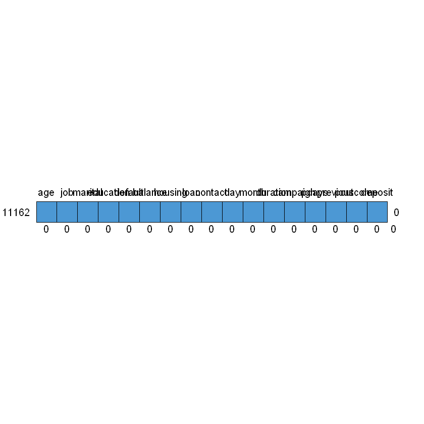
Перевіримо вибірку на наявність пропусків:

suppressMessages(library(mice))
md.pattern(data) # OK

 /\     /\
{  `---'  }
{  O   O  }
==>  V <==  No need for mice. This data set is completely observed.
 \  \|/  /
  `-----'

A matrix: 2 × 18 of type dbl

	age	job	marital	education	default	balance	housing	loan	contact	day	month	duration	campaign	pdays	previous	poutcome	deposit
11162	1	1	1	1	1	1	1	1	1	1	1	1	1	1	1	1	1	0
	0	0	0	0	0	0	0	0	0	0	0	0	0	0	0	0	0	0

anyNA(data)

FALSE

---

7.3 Data visualization

Вік клієнта (age):

library(ggplot2)

ggplot(data, aes(age)) + 
    geom_histogram(bins = 20, alpha = 0.5, fill = 'blue', color='black')  + 
    theme_bw()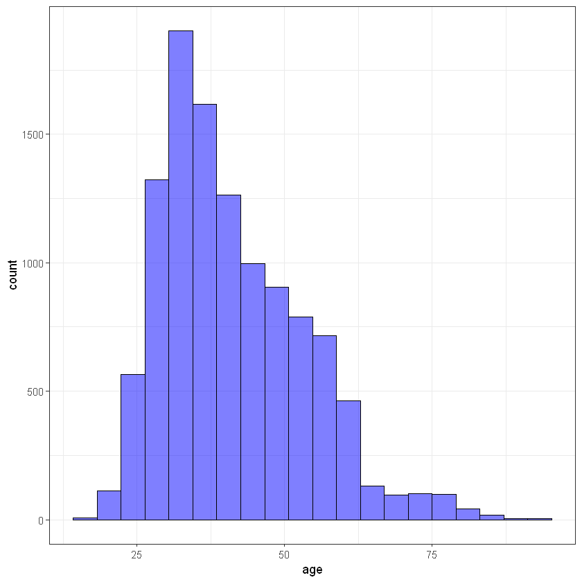

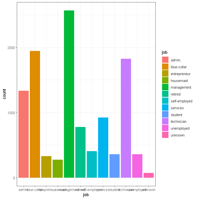
Робота клієнта (job):

ggplot(data, aes(job)) + 
    geom_bar(aes(fill = job)) + 
    theme_bw()

library(gmodels)
CrossTable(data$job, data$deposit)
# more loyal to deposits are management, retired, student, unemployed ))

 
   Cell Contents
|-------------------------|
|                       N |
| Chi-square contribution |
|           N / Row Total |
|           N / Col Total |
|         N / Table Total |
|-------------------------|

 
Total Observations in Table:  11162 

 
              | data$deposit 
     data$job |        no |       yes | Row Total | 
--------------|-----------|-----------|-----------|
       admin. |       703 |       631 |      1334 | 
              |     0.002 |     0.002 |           | 
              |     0.527 |     0.473 |     0.120 | 
              |     0.120 |     0.119 |           | 
              |     0.063 |     0.057 |           | 
--------------|-----------|-----------|-----------|
  blue-collar |      1236 |       708 |      1944 | 
              |    44.415 |    49.320 |           | 
              |     0.636 |     0.364 |     0.174 | 
              |     0.210 |     0.134 |           | 
              |     0.111 |     0.063 |           | 
--------------|-----------|-----------|-----------|
 entrepreneur |       205 |       123 |       328 | 
              |     6.090 |     6.762 |           | 
              |     0.625 |     0.375 |     0.029 | 
              |     0.035 |     0.023 |           | 
              |     0.018 |     0.011 |           | 
--------------|-----------|-----------|-----------|
    housemaid |       165 |       109 |       274 | 
              |     3.010 |     3.343 |           | 
              |     0.602 |     0.398 |     0.025 | 
              |     0.028 |     0.021 |           | 
              |     0.015 |     0.010 |           | 
--------------|-----------|-----------|-----------|
   management |      1265 |      1301 |      2566 | 
              |     5.367 |     5.960 |           | 
              |     0.493 |     0.507 |     0.230 | 
              |     0.215 |     0.246 |           | 
              |     0.113 |     0.117 |           | 
--------------|-----------|-----------|-----------|
      retired |       262 |       516 |       778 | 
              |    53.042 |    58.899 |           | 
              |     0.337 |     0.663 |     0.070 | 
              |     0.045 |     0.098 |           | 
              |     0.023 |     0.046 |           | 
--------------|-----------|-----------|-----------|
self-employed |       218 |       187 |       405 | 
              |     0.113 |     0.125 |           | 
              |     0.538 |     0.462 |     0.036 | 
              |     0.037 |     0.035 |           | 
              |     0.020 |     0.017 |           | 
--------------|-----------|-----------|-----------|
     services |       554 |       369 |       923 | 
              |     9.621 |    10.683 |           | 
              |     0.600 |     0.400 |     0.083 | 
              |     0.094 |     0.070 |           | 
              |     0.050 |     0.033 |           | 
--------------|-----------|-----------|-----------|
      student |        91 |       269 |       360 | 
              |    51.136 |    56.782 |           | 
              |     0.253 |     0.747 |     0.032 | 
              |     0.015 |     0.051 |           | 
              |     0.008 |     0.024 |           | 
--------------|-----------|-----------|-----------|
   technician |       983 |       840 |      1823 | 
              |     0.591 |     0.656 |           | 
              |     0.539 |     0.461 |     0.163 | 
              |     0.167 |     0.159 |           | 
              |     0.088 |     0.075 |           | 
--------------|-----------|-----------|-----------|
   unemployed |       155 |       202 |       357 | 
              |     5.741 |     6.375 |           | 
              |     0.434 |     0.566 |     0.032 | 
              |     0.026 |     0.038 |           | 
              |     0.014 |     0.018 |           | 
--------------|-----------|-----------|-----------|
      unknown |        36 |        34 |        70 | 
              |     0.019 |     0.021 |           | 
              |     0.514 |     0.486 |     0.006 | 
              |     0.006 |     0.006 |           | 
              |     0.003 |     0.003 |           | 
--------------|-----------|-----------|-----------|
 Column Total |      5873 |      5289 |     11162 | 
              |     0.526 |     0.474 |           | 
--------------|-----------|-----------|-----------|

 

Сімейний статус (marital):

ggplot(data, aes(marital)) + 
    geom_bar(aes(fill = marital)) + 
    theme_bw()

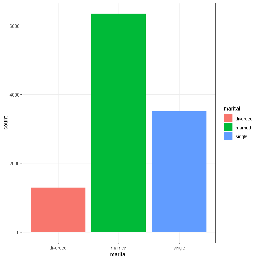
CrossTable(data$marital, data$deposit)
# married are not very loyal to deposits
# but singles is more loyal

 
   Cell Contents
|-------------------------|
|                       N |
| Chi-square contribution |
|           N / Row Total |
|           N / Col Total |
|         N / Table Total |
|-------------------------|

 
Total Observations in Table:  11162 

 
             | data$deposit 
data$marital |        no |       yes | Row Total | 
-------------|-----------|-----------|-----------|
    divorced |       671 |       622 |      1293 | 
             |     0.128 |     0.142 |           | 
             |     0.519 |     0.481 |     0.116 | 
             |     0.114 |     0.118 |           | 
             |     0.060 |     0.056 |           | 
-------------|-----------|-----------|-----------|
     married |      3596 |      2755 |      6351 | 
             |    19.361 |    21.499 |           | 
             |     0.566 |     0.434 |     0.569 | 
             |     0.612 |     0.521 |           | 
             |     0.322 |     0.247 |           | 
-------------|-----------|-----------|-----------|
      single |      1606 |      1912 |      3518 | 
             |    32.436 |    36.018 |           | 
             |     0.457 |     0.543 |     0.315 | 
             |     0.273 |     0.362 |           | 
             |     0.144 |     0.171 |           | 
-------------|-----------|-----------|-----------|
Column Total |      5873 |      5289 |     11162 | 
             |     0.526 |     0.474 |           | 
-------------|-----------|-----------|-----------|

 

Освіта (education):

ggplot(data, aes(education)) + 
    geom_bar(aes(fill = education)) + 
    theme_bw()

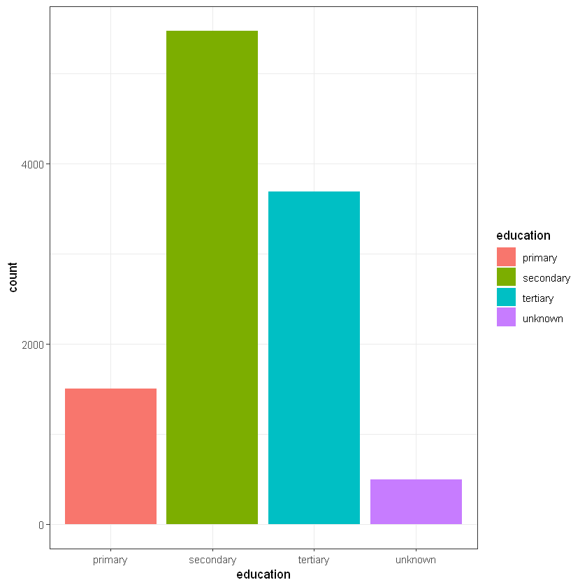
CrossTable(data$education, data$deposit)
# people with tertiary education is more loyal than other groups

 
   Cell Contents
|-------------------------|
|                       N |
| Chi-square contribution |
|           N / Row Total |
|           N / Col Total |
|         N / Table Total |
|-------------------------|

 
Total Observations in Table:  11162 

 
               | data$deposit 
data$education |        no |       yes | Row Total | 
---------------|-----------|-----------|-----------|
       primary |       909 |       591 |      1500 | 
               |    18.172 |    20.179 |           | 
               |     0.606 |     0.394 |     0.134 | 
               |     0.155 |     0.112 |           | 
               |     0.081 |     0.053 |           | 
---------------|-----------|-----------|-----------|
     secondary |      3026 |      2450 |      5476 | 
               |     7.272 |     8.075 |           | 
               |     0.553 |     0.447 |     0.491 | 
               |     0.515 |     0.463 |           | 
               |     0.271 |     0.219 |           | 
---------------|-----------|-----------|-----------|
      tertiary |      1693 |      1996 |      3689 | 
               |    31.688 |    35.187 |           | 
               |     0.459 |     0.541 |     0.330 | 
               |     0.288 |     0.377 |           | 
               |     0.152 |     0.179 |           | 
---------------|-----------|-----------|-----------|
       unknown |       245 |       252 |       497 | 
               |     1.041 |     1.156 |           | 
               |     0.493 |     0.507 |     0.045 | 
               |     0.042 |     0.048 |           | 
               |     0.022 |     0.023 |           | 
---------------|-----------|-----------|-----------|
  Column Total |      5873 |      5289 |     11162 | 
               |     0.526 |     0.474 |           | 
---------------|-----------|-----------|-----------|

 

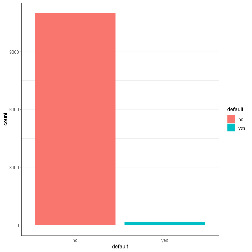
Дефолт (default):

ggplot(data, aes(default)) + 
    geom_bar(aes(fill = default)) + 
    theme_bw()

CrossTable(data$default, data$deposit)
# defaults not very loyal to deposits, but why? ))))))

 
   Cell Contents
|-------------------------|
|                       N |
| Chi-square contribution |
|           N / Row Total |
|           N / Col Total |
|         N / Table Total |
|-------------------------|

 
Total Observations in Table:  11162 

 
             | data$deposit 
data$default |        no |       yes | Row Total | 
-------------|-----------|-----------|-----------|
          no |      5757 |      5237 |     10994 | 
             |     0.132 |     0.146 |           | 
             |     0.524 |     0.476 |     0.985 | 
             |     0.980 |     0.990 |           | 
             |     0.516 |     0.469 |           | 
-------------|-----------|-----------|-----------|
         yes |       116 |        52 |       168 | 
             |     8.621 |     9.573 |           | 
             |     0.690 |     0.310 |     0.015 | 
             |     0.020 |     0.010 |           | 
             |     0.010 |     0.005 |           | 
-------------|-----------|-----------|-----------|
Column Total |      5873 |      5289 |     11162 | 
             |     0.526 |     0.474 |           | 
-------------|-----------|-----------|-----------|

 

Баланс (balance):

ggplot(data, aes(balance)) + 
    geom_histogram(bins = 30, alpha = 0.5, fill = 'blue', color='black')  + 
    theme_bw()

# looks like balance data has outliers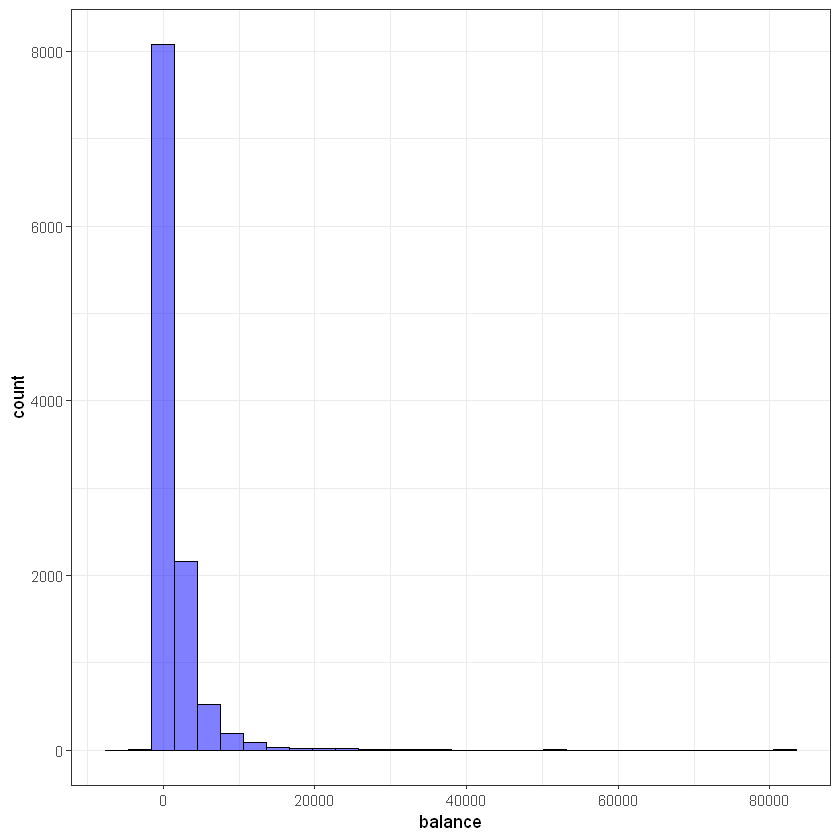

Наявність кредиту на житло (housing):

ggplot(data, aes(housing)) + 
    geom_bar(aes(fill = housing)) + 
    theme_bw()

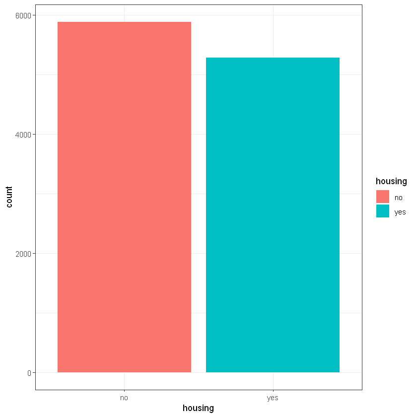
CrossTable(data$housing, data$deposit)
# people without housing load logicaly more often can do deposits

 
   Cell Contents
|-------------------------|
|                       N |
| Chi-square contribution |
|           N / Row Total |
|           N / Col Total |
|         N / Table Total |
|-------------------------|

 
Total Observations in Table:  11162 

 
             | data$deposit 
data$housing |        no |       yes | Row Total | 
-------------|-----------|-----------|-----------|
          no |      2527 |      3354 |      5881 | 
             |   104.023 |   115.509 |           | 
             |     0.430 |     0.570 |     0.527 | 
             |     0.430 |     0.634 |           | 
             |     0.226 |     0.300 |           | 
-------------|-----------|-----------|-----------|
         yes |      3346 |      1935 |      5281 | 
             |   115.842 |   128.633 |           | 
             |     0.634 |     0.366 |     0.473 | 
             |     0.570 |     0.366 |           | 
             |     0.300 |     0.173 |           | 
-------------|-----------|-----------|-----------|
Column Total |      5873 |      5289 |     11162 | 
             |     0.526 |     0.474 |           | 
-------------|-----------|-----------|-----------|

 

Наявність позики (loan):

ggplot(data, aes(loan)) + 
    geom_bar(aes(fill = loan)) + 
    theme_bw()

CrossTable(data$loan, data$deposit)

 
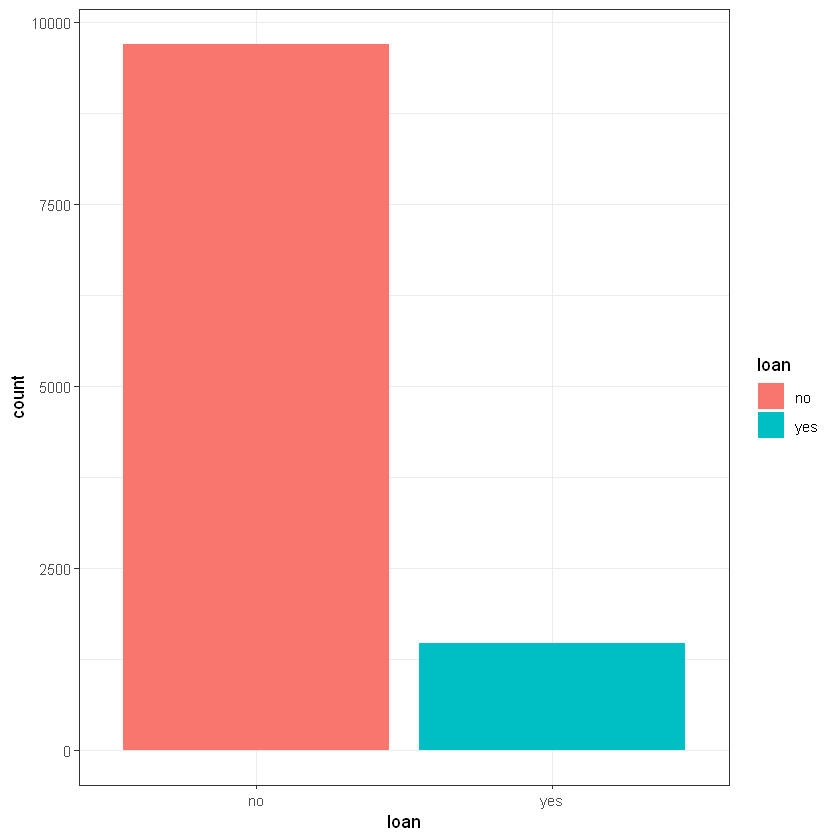
   Cell Contents
|-------------------------|
|                       N |
| Chi-square contribution |
|           N / Row Total |
|           N / Col Total |
|         N / Table Total |
|-------------------------|

 
Total Observations in Table:  11162 

 
             | data$deposit 
   data$loan |        no |       yes | Row Total | 
-------------|-----------|-----------|-----------|
          no |      4897 |      4805 |      9702 | 
             |     8.459 |     9.393 |           | 
             |     0.505 |     0.495 |     0.869 | 
             |     0.834 |     0.908 |           | 
             |     0.439 |     0.430 |           | 
-------------|-----------|-----------|-----------|
         yes |       976 |       484 |      1460 | 
             |    56.214 |    62.421 |           | 
             |     0.668 |     0.332 |     0.131 | 
             |     0.166 |     0.092 |           | 
             |     0.087 |     0.043 |           | 
-------------|-----------|-----------|-----------|
Column Total |      5873 |      5289 |     11162 | 
             |     0.526 |     0.474 |           | 
-------------|-----------|-----------|-----------|

 

# Тип комунікації (contact):

ggplot(data, aes(contact)) + 
    geom_bar(aes(fill = contact)) + 
    theme_bw()

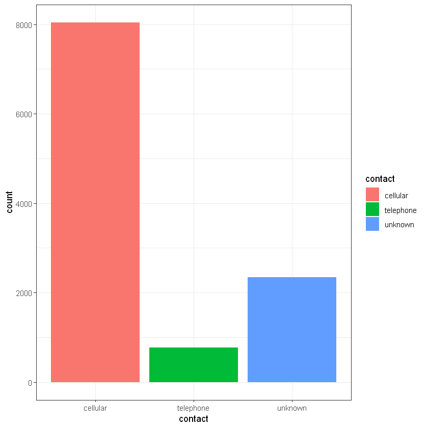
CrossTable(data$contact, data$deposit)
# cellular communication channel looks like the best way to increase deposits count
# people with cellular devices has more money? 

 
   Cell Contents
|-------------------------|
|                       N |
| Chi-square contribution |
|           N / Row Total |
|           N / Col Total |
|         N / Table Total |
|-------------------------|

 
Total Observations in Table:  11162 

 
             | data$deposit 
data$contact |        no |       yes | Row Total | 
-------------|-----------|-----------|-----------|
    cellular |      3673 |      4369 |      8042 | 
             |    73.685 |    81.821 |           | 
             |     0.457 |     0.543 |     0.720 | 
             |     0.625 |     0.826 |           | 
             |     0.329 |     0.391 |           | 
-------------|-----------|-----------|-----------|
   telephone |       384 |       390 |       774 | 
             |     1.327 |     1.474 |           | 
             |     0.496 |     0.504 |     0.069 | 
             |     0.065 |     0.074 |           | 
             |     0.034 |     0.035 |           | 
-------------|-----------|-----------|-----------|
     unknown |      1816 |       530 |      2346 | 
             |   274.060 |   304.321 |           | 
             |     0.774 |     0.226 |     0.210 | 
             |     0.309 |     0.100 |           | 
             |     0.163 |     0.047 |           | 
-------------|-----------|-----------|-----------|
Column Total |      5873 |      5289 |     11162 | 
             |     0.526 |     0.474 |           | 
-------------|-----------|-----------|-----------|

 

День місяця (day):

ggplot(data, aes(day)) + 
    geom_histogram(bins = 25, alpha = 0.5, fill = 'blue', color='black')  + 
    theme_bw()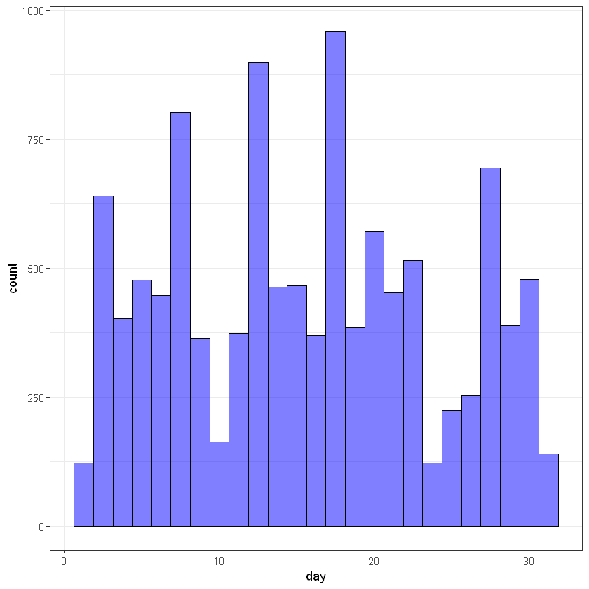

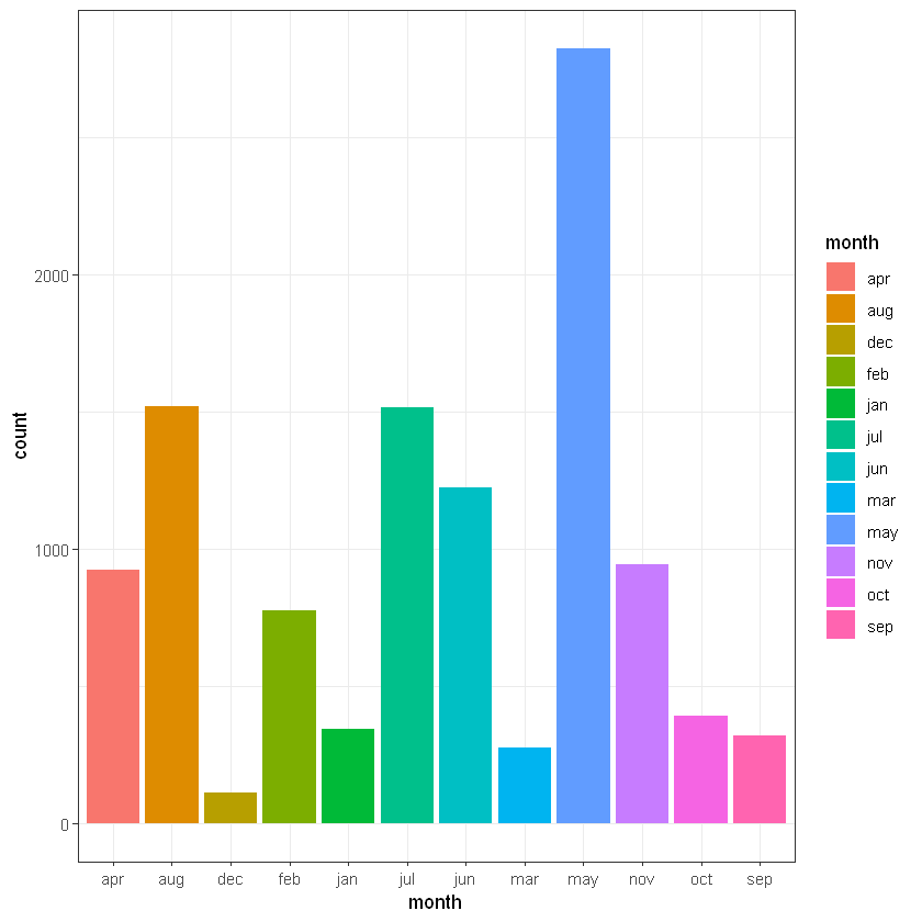
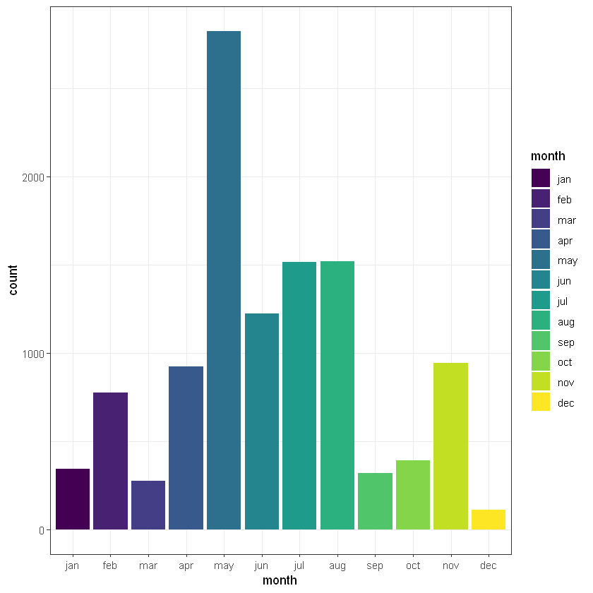
Місяць (month):

ggplot(data, aes(month)) + 
    geom_bar(aes(fill = month)) + 
    theme_bw()

# So, lets replace our month with ordered factor for correct visualization
suppressMessages(library(dplyr))
data <- data |>
    mutate(month = factor(month, levels=c("jan","feb","mar",
               "apr","may","jun","jul","aug","sep",
              "oct","nov","dec"),ordered=TRUE))

ggplot(data, aes(month)) + 
    geom_bar(aes(fill = month)) + 
    theme_bw()

CrossTable(data$month, data$deposit)

 
   Cell Contents
|-------------------------|
|                       N |
| Chi-square contribution |
|           N / Row Total |
|           N / Col Total |
|         N / Table Total |
|-------------------------|

 
Total Observations in Table:  11162 

 
             | data$deposit 
  data$month |        no |       yes | Row Total | 
-------------|-----------|-----------|-----------|
         jan |       202 |       142 |       344 | 
             |     2.437 |     2.706 |           | 
             |     0.587 |     0.413 |     0.031 | 
             |     0.034 |     0.027 |           | 
             |     0.018 |     0.013 |           | 
-------------|-----------|-----------|-----------|
         feb |       335 |       441 |       776 | 
             |    13.159 |    14.612 |           | 
             |     0.432 |     0.568 |     0.070 | 
             |     0.057 |     0.083 |           | 
             |     0.030 |     0.040 |           | 
-------------|-----------|-----------|-----------|
         mar |        28 |       248 |       276 | 
             |    94.619 |   105.067 |           | 
             |     0.101 |     0.899 |     0.025 | 
             |     0.005 |     0.047 |           | 
             |     0.003 |     0.022 |           | 
-------------|-----------|-----------|-----------|
         apr |       346 |       577 |       923 | 
             |    40.155 |    44.588 |           | 
             |     0.375 |     0.625 |     0.083 | 
             |     0.059 |     0.109 |           | 
             |     0.031 |     0.052 |           | 
-------------|-----------|-----------|-----------|
         may |      1899 |       925 |      2824 | 
             |   114.862 |   127.545 |           | 
             |     0.672 |     0.328 |     0.253 | 
             |     0.323 |     0.175 |           | 
             |     0.170 |     0.083 |           | 
-------------|-----------|-----------|-----------|
         jun |       676 |       546 |      1222 | 
             |     1.697 |     1.884 |           | 
             |     0.553 |     0.447 |     0.109 | 
             |     0.115 |     0.103 |           | 
             |     0.061 |     0.049 |           | 
-------------|-----------|-----------|-----------|
         jul |       887 |       627 |      1514 | 
             |    10.257 |    11.390 |           | 
             |     0.586 |     0.414 |     0.136 | 
             |     0.151 |     0.119 |           | 
             |     0.079 |     0.056 |           | 
-------------|-----------|-----------|-----------|
         aug |       831 |       688 |      1519 | 
             |     1.262 |     1.402 |           | 
             |     0.547 |     0.453 |     0.136 | 
             |     0.141 |     0.130 |           | 
             |     0.074 |     0.062 |           | 
-------------|-----------|-----------|-----------|
         sep |        50 |       269 |       319 | 
             |    82.740 |    91.876 |           | 
             |     0.157 |     0.843 |     0.029 | 
             |     0.009 |     0.051 |           | 
             |     0.004 |     0.024 |           | 
-------------|-----------|-----------|-----------|
         oct |        69 |       323 |       392 | 
             |    91.338 |   101.423 |           | 
             |     0.176 |     0.824 |     0.035 | 
             |     0.012 |     0.061 |           | 
             |     0.006 |     0.029 |           | 
-------------|-----------|-----------|-----------|
         nov |       540 |       403 |       943 | 
             |     3.872 |     4.300 |           | 
             |     0.573 |     0.427 |     0.084 | 
             |     0.092 |     0.076 |           | 
             |     0.048 |     0.036 |           | 
-------------|-----------|-----------|-----------|
         dec |        10 |       100 |       110 | 
             |    39.605 |    43.979 |           | 
             |     0.091 |     0.909 |     0.010 | 
             |     0.002 |     0.019 |           | 
             |     0.001 |     0.009 |           | 
-------------|-----------|-----------|-----------|
Column Total |      5873 |      5289 |     11162 | 
             |     0.526 |     0.474 |           | 
-------------|-----------|-----------|-----------|

 

Тривалість останнього контакту (duration):

ggplot(data, aes(duration)) + 
    geom_histogram(bins = 100, alpha = 0.5, fill = 'blue', color='black')  + 
    theme_bw()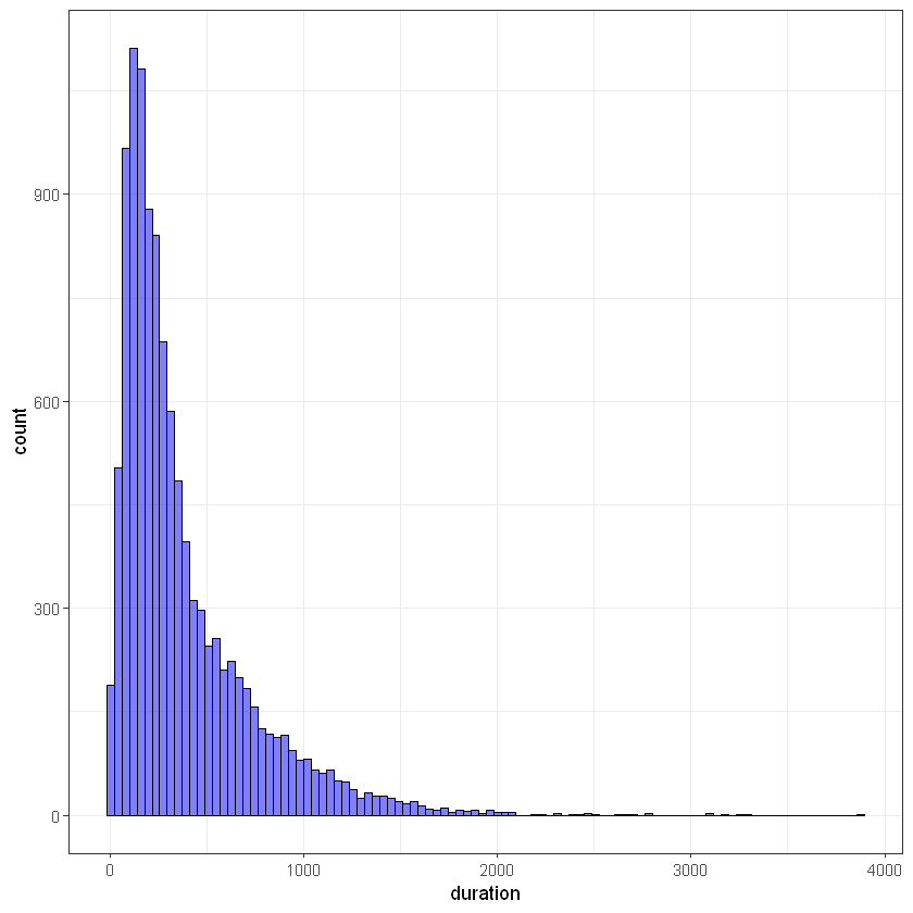

Кількість контактів протягом поточної кампанії (campaign):

ggplot(data, aes(campaign)) + 
    geom_histogram(bins = 30, alpha = 0.5, fill = 'blue', color='black')  + 
    theme_bw()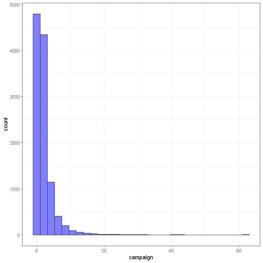

Кількість днів від попередньої акції (pday):

ggplot(data, aes(pdays)) + 
    geom_histogram(bins = 20, alpha = 0.5, fill = 'blue', color='black')  + 
    theme_bw()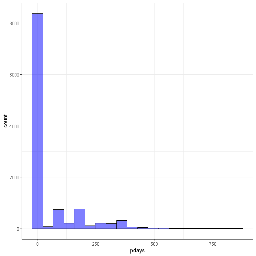

Кількість контактів до початку поточної кампанії (previous):

ggplot(data, aes(previous)) + 
    geom_histogram(bins = 50, alpha = 0.5, fill = 'blue', color='black')  + 
    theme_bw()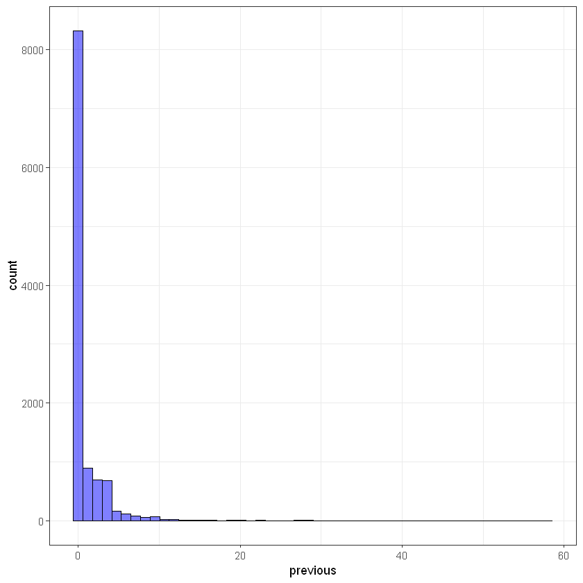

Результат попередньої кампанії (poutcome):

ggplot(data, aes(poutcome)) + 
    geom_bar(aes(fill = poutcome)) + 
    theme_bw()

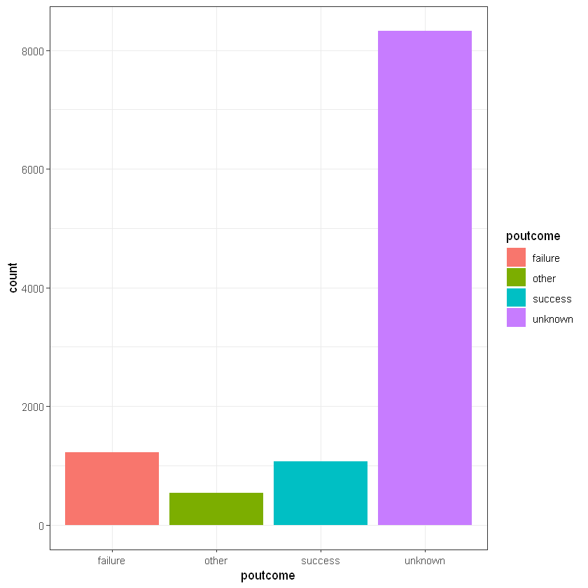
CrossTable(data$poutcome, data$deposit)
# people with previous success status also loyal for new propositions

 
   Cell Contents
|-------------------------|
|                       N |
| Chi-square contribution |
|           N / Row Total |
|           N / Col Total |
|         N / Table Total |
|-------------------------|

 
Total Observations in Table:  11162 

 
              | data$deposit 
data$poutcome |        no |       yes | Row Total | 
--------------|-----------|-----------|-----------|
      failure |       610 |       618 |      1228 | 
              |     2.020 |     2.243 |           | 
              |     0.497 |     0.503 |     0.110 | 
              |     0.104 |     0.117 |           | 
              |     0.055 |     0.055 |           | 
--------------|-----------|-----------|-----------|
        other |       230 |       307 |       537 | 
              |     9.773 |    10.852 |           | 
              |     0.428 |     0.572 |     0.048 | 
              |     0.039 |     0.058 |           | 
              |     0.021 |     0.028 |           | 
--------------|-----------|-----------|-----------|
      success |        93 |       978 |      1071 | 
              |   392.866 |   436.245 |           | 
              |     0.087 |     0.913 |     0.096 | 
              |     0.016 |     0.185 |           | 
              |     0.008 |     0.088 |           | 
--------------|-----------|-----------|-----------|
      unknown |      4940 |      3386 |      8326 | 
              |    71.378 |    79.259 |           | 
              |     0.593 |     0.407 |     0.746 | 
              |     0.841 |     0.640 |           | 
              |     0.443 |     0.303 |           | 
--------------|-----------|-----------|-----------|
 Column Total |      5873 |      5289 |     11162 | 
              |     0.526 |     0.474 |           | 
--------------|-----------|-----------|-----------|

 

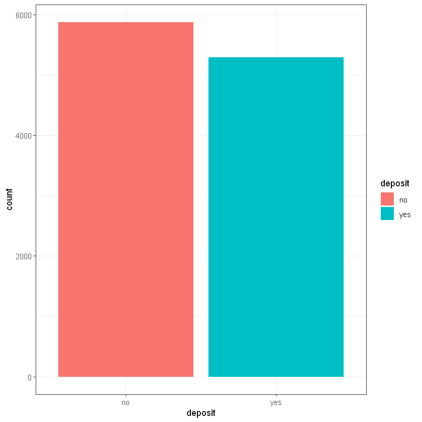
Результат укладання або відсутність укладання договору (deposit):

ggplot(data, aes(deposit)) + 
    geom_bar(aes(fill = deposit)) + 
    theme_bw()

CrossTable(data$deposit)

 
   Cell Contents
|-------------------------|
|                       N |
|         N / Table Total |
|-------------------------|

 
Total Observations in Table:  11162 

 
          |        no |       yes | 
          |-----------|-----------|
          |      5873 |      5289 | 
          |     0.526 |     0.474 | 
          |-----------|-----------|



 

7.4 Data preprocessing

Перетворимо значення deposit до 0 і 1:

data$deposit <- ifelse(data$deposit == "yes", 1, 0)

Видалимо duration, адже цей параметр чітко вказує на факт укладання угоди, такі дані називаються leak:

data$duration <- NULL

Створимо новий параметр pdays_flag, який вказує чи був контакт з клієнтом раніше:

data$pdays_flag <- ifelse(data$pdays > 0, 1, 0)

head(data)

A data.frame: 6 × 17

	age	job	marital	education	default	balance	housing	loan	contact	day	month	campaign	pdays	previous	poutcome	deposit	pdays_flag
	<int>	<fct>	<fct>	<fct>	<fct>	<int>	<fct>	<fct>	<fct>	<int>	<ord>	<int>	<int>	<int>	<fct>	<dbl>	<dbl>
1	59	admin.	married	secondary	no	2343	yes	no	unknown	5	may	1	-1	0	unknown	1	0
2	56	admin.	married	secondary	no	45	no	no	unknown	5	may	1	-1	0	unknown	1	0
3	41	technician	married	secondary	no	1270	yes	no	unknown	5	may	1	-1	0	unknown	1	0
4	55	services	married	secondary	no	2476	yes	no	unknown	5	may	1	-1	0	unknown	1	0
5	54	admin.	married	tertiary	no	184	no	no	unknown	5	may	2	-1	0	unknown	1	0
6	42	management	single	tertiary	no	0	yes	yes	unknown	5	may	2	-1	0	unknown	1	0

Створимо новий параметр poutcome_success, який вказує чи була попередня кампанія з цим клієнтом “успішною для банку”:

data$poutcoume_success <- ifelse(data$poutcome == "success", 1, 0)

---

7.5 Train/test split

Задаємо seed для генератора випадкових чисел

Train 65%, test 35%

set.seed(111) 
suppressMessages(library(caret))
index = createDataPartition(data$deposit, p = 0.65, list = FALSE)
train_data = data[index, ]
test_data = data[-index, ]

CrossTable(train_data$deposit)
CrossTable(test_data$deposit)

 
   Cell Contents
|-------------------------|
|                       N |
|         N / Table Total |
|-------------------------|

 
Total Observations in Table:  7256 

 
          |         0 |         1 | 
          |-----------|-----------|
          |      3816 |      3440 | 
          |     0.526 |     0.474 | 
          |-----------|-----------|



 

 
   Cell Contents
|-------------------------|
|                       N |
|         N / Table Total |
|-------------------------|

 
Total Observations in Table:  3906 

 
          |         0 |         1 | 
          |-----------|-----------|
          |      2057 |      1849 | 
          |     0.527 |     0.473 | 
          |-----------|-----------|



 

---

7.6 Decision trees with rpart()

Для побудови дерев рішень у R є ряд пакетів та алгоритмів. Розглянемо пакет rpart.

#install.packages("rpart")
library(rpart)
rpart_model <- rpart(deposit ~ ., train_data)

Виведемо опис моделі:

rpart_model

n= 7256 

node), split, n, deviance, yval
      * denotes terminal node

 1) root 7256 1809.12900 0.4740904  
   2) poutcome=failure,other,unknown 6563 1605.86300 0.4270913  
     4) contact=unknown 1543  272.24240 0.2287751 *
     5) contact=cellular,telephone 5020 1254.28300 0.4880478  
      10) housing=yes 2139  507.93360 0.3880318 *
      11) housing=no 2881  709.06630 0.5623048  
        22) balance< 105.5 636  150.38990 0.3836478 *
        23) balance>=105.5 2245  532.62540 0.6129176 *
   3) poutcome=success 693   51.47475 0.9191919 *

Дуже детальний опис:

summary(rpart_model)

Call:
rpart(formula = deposit ~ ., data = train_data)
  n= 7256 

          CP nsplit rel error    xerror        xstd
1 0.08390285      0 1.0000000 1.0004337 0.001224021
2 0.04385421      1 0.9160972 0.9165627 0.005207633
3 0.02060824      2 0.8722429 0.8731088 0.006530786
4 0.01439973      3 0.8516347 0.8528095 0.007275812
5 0.01000000      4 0.8372350 0.8459897 0.007777416

Variable importance
         poutcome poutcoume_success           contact           housing 
               33                33                17                 8 
          balance               job             pdays             month 
                6                 1                 1                 1 

Node number 1: 7256 observations,    complexity param=0.08390285
  mean=0.4740904, MSE=0.2493287 
  left son=2 (6563 obs) right son=3 (693 obs)
  Primary splits:
      poutcome          splits as  LLRL,      improve=0.08390285, (0 missing)
      poutcoume_success < 0.5   to the left,  improve=0.08390285, (0 missing)
      contact           splits as  RRL,       improve=0.06524266, (0 missing)
      pdays             < 9.5   to the left,  improve=0.04926922, (0 missing)
      previous          < 0.5   to the left,  improve=0.04820004, (0 missing)
  Surrogate splits:
      poutcoume_success < 0.5   to the left,  agree=1.000, adj=1.000, (0 split)
      age               < 91    to the left,  agree=0.905, adj=0.003, (0 split)

Node number 2: 6563 observations,    complexity param=0.04385421
  mean=0.4270913, MSE=0.2446843 
  left son=4 (1543 obs) right son=5 (5020 obs)
  Primary splits:
      contact splits as  RRL,          improve=0.04940515, (0 missing)
      housing splits as  RL,           improve=0.03656129, (0 missing)
      age     < 60.5  to the left,     improve=0.02289822, (0 missing)
      job     splits as  LLLLLRLLRLRL, improve=0.02007437, (0 missing)
      balance < 798   to the left,     improve=0.01917691, (0 missing)
  Surrogate splits:
      campaign < 24.5  to the right, agree=0.766, adj=0.003, (0 split)

Node number 3: 693 observations
  mean=0.9191919, MSE=0.07427813 

Node number 4: 1543 observations
  mean=0.2287751, MSE=0.1764371 

Node number 5: 5020 observations,    complexity param=0.02060824
  mean=0.4880478, MSE=0.2498571 
  left son=10 (2139 obs) right son=11 (2881 obs)
  Primary splits:
      housing splits as  RL,           improve=0.02972452, (0 missing)
      balance < 799.5 to the left,     improve=0.02236410, (0 missing)
      job     splits as  LLLLLRLLRLRL, improve=0.02093907, (0 missing)
      age     < 59.5  to the left,     improve=0.02067340, (0 missing)
      loan    splits as  RL,           improve=0.01407420, (0 missing)
  Surrogate splits:
      job      splits as  LLRRRRRLRRRR, agree=0.630, adj=0.132, (0 split)
      pdays    < 165.5 to the right,    agree=0.623, adj=0.115, (0 split)
      month    splits as  LLLLLRRRRRRR, agree=0.615, adj=0.096, (0 split)
      poutcome splits as  LR-R,         agree=0.604, adj=0.071, (0 split)
      previous < 0.5   to the right,    agree=0.599, adj=0.059, (0 split)

Node number 10: 2139 observations
  mean=0.3880318, MSE=0.2374631 

Node number 11: 2881 observations,    complexity param=0.01439973
  mean=0.5623048, MSE=0.2461181 
  left son=22 (636 obs) right son=23 (2245 obs)
  Primary splits:
      balance < 105.5 to the left,     improve=0.03673982, (0 missing)
      loan    splits as  RL,           improve=0.03447328, (0 missing)
      month   splits as  RRRRRRLLLLLL, improve=0.03024729, (0 missing)
      job     splits as  LLLLLRLLRLRL, improve=0.02005774, (0 missing)
      age     < 60.5  to the left,     improve=0.01886179, (0 missing)
  Surrogate splits:
      default splits as  RL, agree=0.787, adj=0.035, (0 split)

Node number 22: 636 observations
  mean=0.3836478, MSE=0.2364622 

Node number 23: 2245 observations
  mean=0.6129176, MSE=0.2372496 

Візуалізуємо дерево рішень:

# install.packages(c("rattle", "RColorBrewer"))

suppressMessages(library(rattle))
suppressMessages(library(RColorBrewer))
fancyRpartPlot(rpart_model)

# now you can see how model model works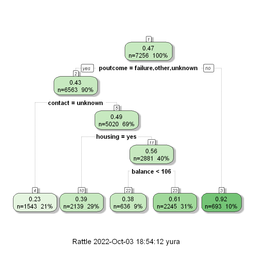

Створимо два дата-фрейм для для запису результатів моделювання на тестовій вибірці. Одразу додамо у набори даних реальні значення результатів маркетингової акції deposit та модельовані значення

Дані тренувальної вибірки будуть використовуватися для визначення оптимальної cutoff лінії, а тестової для порівняння моделей між собою.

train_results <- data.frame(No = c(1:nrow(train_data)), 
                            deposit = train_data$deposit, 
                            RPartPredicted = predict(rpart_model, train_data))

test_results <- data.frame(No = c(1:nrow(test_data)),
                           deposit = test_data$deposit, 
                           RPartPredicted = predict(rpart_model, test_data))

head(test_results)

A data.frame: 6 × 3

	No	deposit	RPartPredicted
	<int>	<dbl>	<dbl>
1	1	1	0.2287751
2	2	1	0.2287751
4	3	1	0.2287751
7	4	1	0.2287751
8	5	1	0.2287751
9	6	1	0.2287751

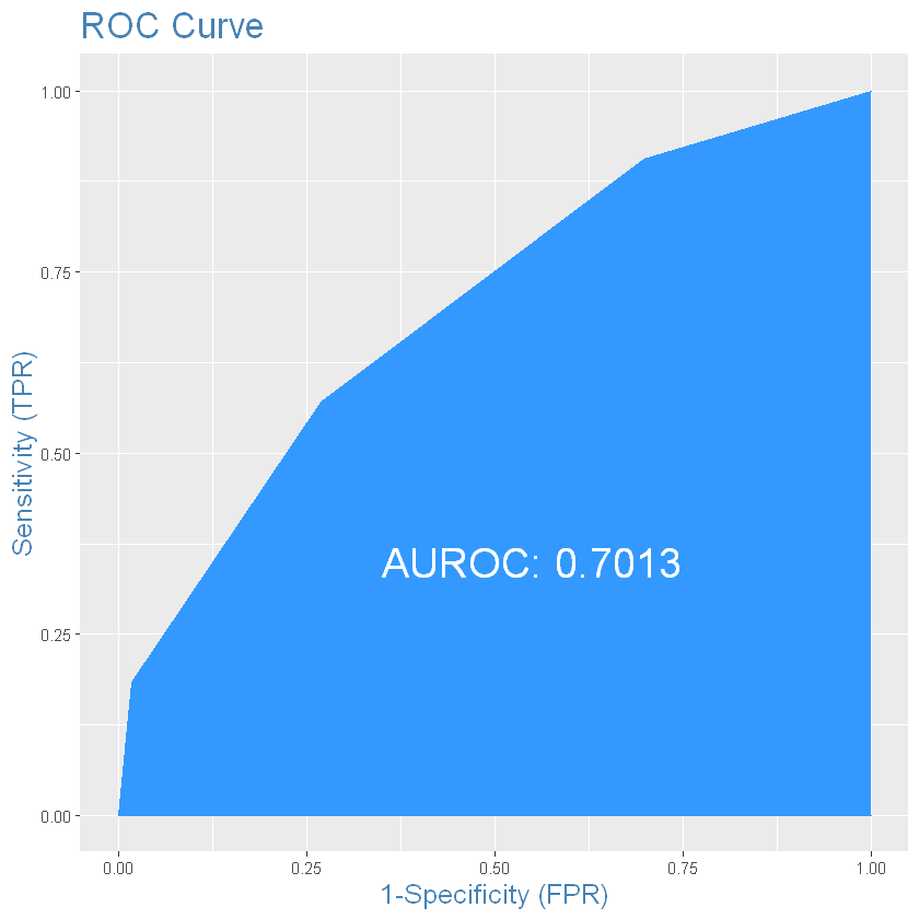
Визначимо оптимальну лінію розподілу на 0 і 1 для тренувальної вибірки за допомогою пакету InformationValue:

suppressMessages(library(InformationValue))
optCutOff <- optimalCutoff(train_results$deposit, train_results$RPartPredicted)
optCutOff

0.389191919191919

Побудуємо ROC-криву для тестової вибірки:

plotROC(test_results$deposit, test_results$RPartPredicted)

Сформуємо набір класів 0 і 1 для тестового набору даних:

test_results$RPartPredicted_Class <- ifelse(test_results$RPartPredicted > optCutOff, 1, 0)

Confusion matrix:

cm <- caret::confusionMatrix(factor(test_results$deposit), 
                      factor(test_results$RPartPredicted_Class), 
                      positive = "1")
cm

Confusion Matrix and Statistics

          Reference
Prediction    0    1
         0 1504  553
         1  793 1056
                                          
               Accuracy : 0.6554          
                 95% CI : (0.6403, 0.6703)
    No Information Rate : 0.5881          
    P-Value [Acc > NIR] : < 2.2e-16       
                                          
                  Kappa : 0.3043          
                                          
 Mcnemar's Test P-Value : 7.297e-11       
                                          
            Sensitivity : 0.6563          
            Specificity : 0.6548          
         Pos Pred Value : 0.5711          
         Neg Pred Value : 0.7312          
             Prevalence : 0.4119          
         Detection Rate : 0.2704          
   Detection Prevalence : 0.4734          
      Balanced Accuracy : 0.6555          
                                          
       'Positive' Class : 1               
                                          

Переглянемо збалансовану точність класифіції:

BAcc <- cm$byClass[["Balanced Accuracy"]]
BAcc 

0.655537676754586

---

7.7 Desicion trees with PartyKit

Побудуємо дерево рішень за допоомгою пакету partykit:

#install.packages("partykit")
suppressMessages(library(partykit))
head(train_data)
party_model <- ctree(deposit ~ ., data = train_data)

A data.frame: 6 × 18

	age	job	marital	education	default	balance	housing	loan	contact	day	month	campaign	pdays	previous	poutcome	deposit	pdays_flag	poutcoume_success
	<int>	<fct>	<fct>	<fct>	<fct>	<int>	<fct>	<fct>	<fct>	<int>	<ord>	<int>	<int>	<int>	<fct>	<dbl>	<dbl>	<dbl>
3	41	technician	married	secondary	no	1270	yes	no	unknown	5	may	1	-1	0	unknown	1	0	0
5	54	admin.	married	tertiary	no	184	no	no	unknown	5	may	2	-1	0	unknown	1	0	0
6	42	management	single	tertiary	no	0	yes	yes	unknown	5	may	2	-1	0	unknown	1	0	0
11	38	admin.	single	secondary	no	100	yes	no	unknown	7	may	1	-1	0	unknown	1	0	0
12	30	blue-collar	married	secondary	no	309	yes	no	unknown	7	may	2	-1	0	unknown	1	0	0
14	46	blue-collar	single	tertiary	no	460	yes	no	unknown	7	may	2	-1	0	unknown	1	0	0

Виведемо текстовий опис моделі:

party_model
# Looks like this model is more complex

Model formula:
deposit ~ age + job + marital + education + default + balance + 
    housing + loan + contact + day + month + campaign + pdays + 
    previous + poutcome + pdays_flag + poutcoume_success

Fitted party:
[1] root
|   [2] poutcome in failure, other, unknown
|   |   [3] contact in cellular, telephone
|   |   |   [4] housing in no
|   |   |   |   [5] loan in no
|   |   |   |   |   [6] campaign <= 3
|   |   |   |   |   |   [7] job in admin., management, retired, student, unemployed
|   |   |   |   |   |   |   [8] day <= 17: 0.733 (n = 715, err = 140.0)
|   |   |   |   |   |   |   [9] day > 17
|   |   |   |   |   |   |   |   [10] job in admin., management, retired, unemployed: 0.583 (n = 434, err = 105.5)
|   |   |   |   |   |   |   |   [11] job in student: 0.843 (n = 51, err = 6.7)
|   |   |   |   |   |   [12] job in blue-collar, entrepreneur, housemaid, self-employed, services, technician, unknown
|   |   |   |   |   |   |   [13] campaign <= 1: 0.612 (n = 415, err = 98.5)
|   |   |   |   |   |   |   [14] campaign > 1
|   |   |   |   |   |   |   |   [15] balance <= 106
|   |   |   |   |   |   |   |   |   [16] age <= 57: 0.234 (n = 94, err = 16.9)
|   |   |   |   |   |   |   |   |   [17] age > 57: 0.700 (n = 10, err = 2.1)
|   |   |   |   |   |   |   |   [18] balance > 106: 0.561 (n = 321, err = 79.1)
|   |   |   |   |   [19] campaign > 3
|   |   |   |   |   |   [20] marital in divorced, single: 0.579 (n = 195, err = 47.5)
|   |   |   |   |   |   [21] marital in married
|   |   |   |   |   |   |   [22] campaign <= 5: 0.474 (n = 171, err = 42.6)
|   |   |   |   |   |   |   [23] campaign > 5: 0.299 (n = 154, err = 32.3)
|   |   |   |   [24] loan in yes: 0.302 (n = 321, err = 67.7)
|   |   |   [25] housing in yes
|   |   |   |   [26] campaign <= 3
|   |   |   |   |   [27] marital in divorced, single: 0.455 (n = 759, err = 188.2)
|   |   |   |   |   [28] marital in married: 0.372 (n = 985, err = 230.0)
|   |   |   |   [29] campaign > 3: 0.301 (n = 395, err = 83.1)
|   |   [30] contact in unknown
|   |   |   [31] month <= sep
|   |   |   |   [32] marital in divorced, single: 0.275 (n = 619, err = 123.3)
|   |   |   |   [33] marital in married: 0.183 (n = 903, err = 134.9)
|   |   |   [34] month > sep: 0.857 (n = 21, err = 2.6)
|   [35] poutcome in success
|   |   [36] contact in cellular: 0.925 (n = 637, err = 44.4)
|   |   [37] contact in telephone, unknown: 0.857 (n = 56, err = 6.9)

Number of inner nodes:    18
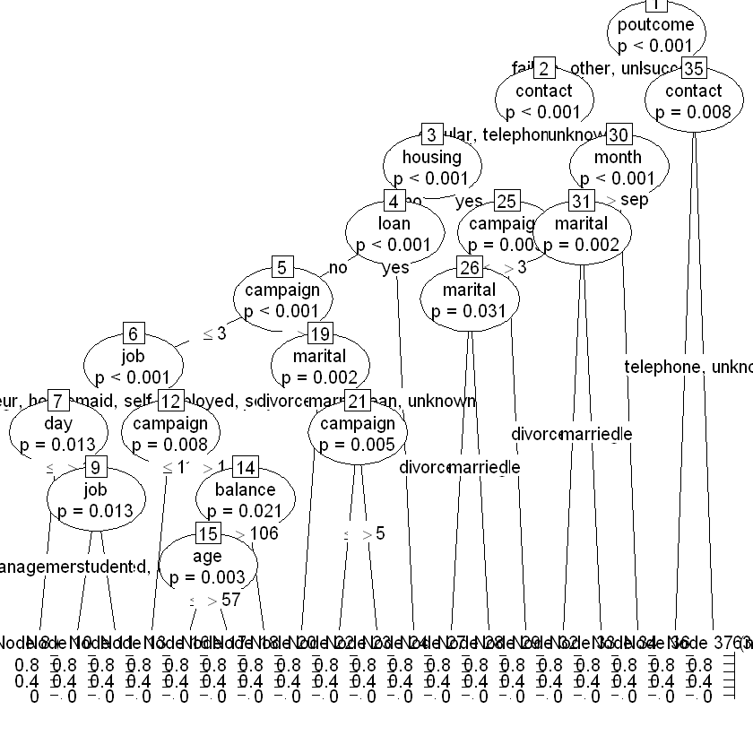
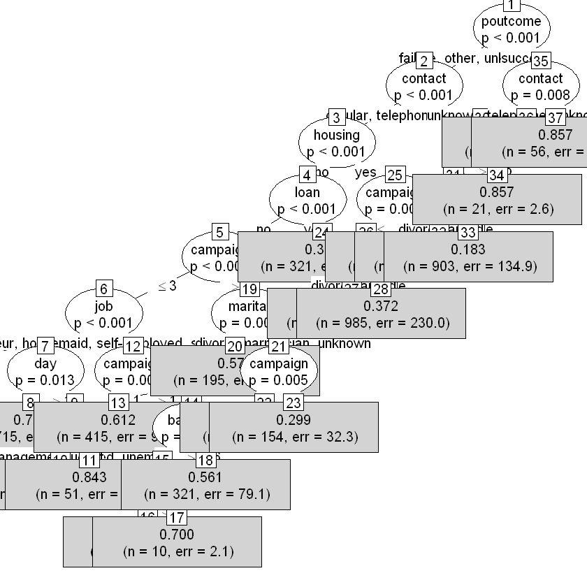
Number of terminal nodes: 19

Візуалізуємо побудоване дерево рішень:

plot(party_model)

Конвернтуємо ctree() до rpart():

st <- as.simpleparty(party_model)
plot(st)

Додамо прогнозовані показники до раніше створених дата-фрейму для збору результатів:

train_results$PartyPredicted <- predict(party_model, train_data)
test_results$PartyPredicted <- predict(party_model, test_data)
head(test_results)

A data.frame: 6 × 5

	No	deposit	RPartPredicted	RPartPredicted_Class	PartyPredicted
	<int>	<dbl>	<dbl>	<dbl>	<dbl>
1	1	1	0.2287751	0	0.1827243
2	2	1	0.2287751	0	0.1827243
4	3	1	0.2287751	0	0.1827243
7	4	1	0.2287751	0	0.1827243
8	5	1	0.2287751	0	0.2746365
9	6	1	0.2287751	0	0.1827243

Визначимо оптимальну лінію розділення на класи 0 і 1:

optCutOff <- optimalCutoff(train_results$deposit, train_results$PartyPredicted)
optCutOff

0.474646781789639

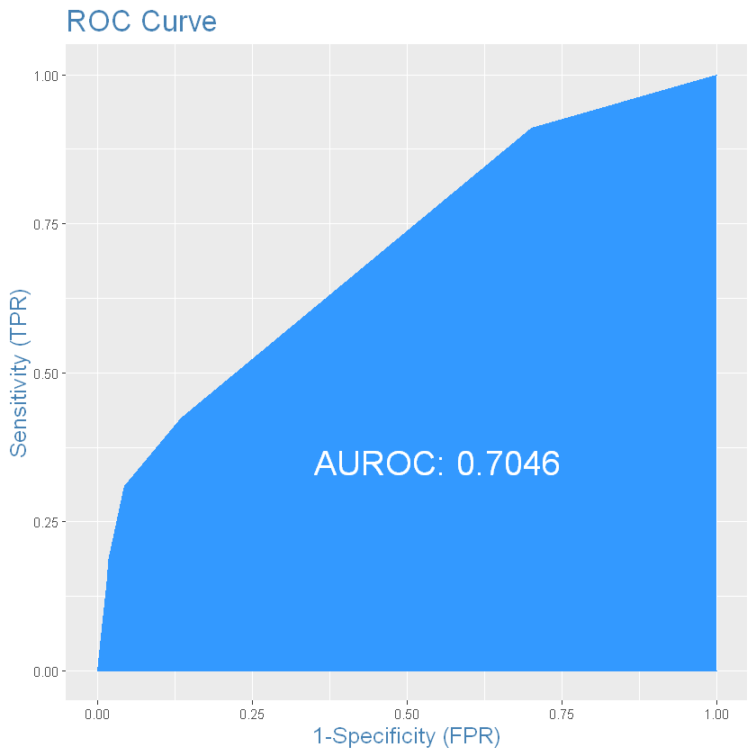
ROC-крива та AUROC:

plotROC(test_results$deposit, test_results$PartyPredicted)

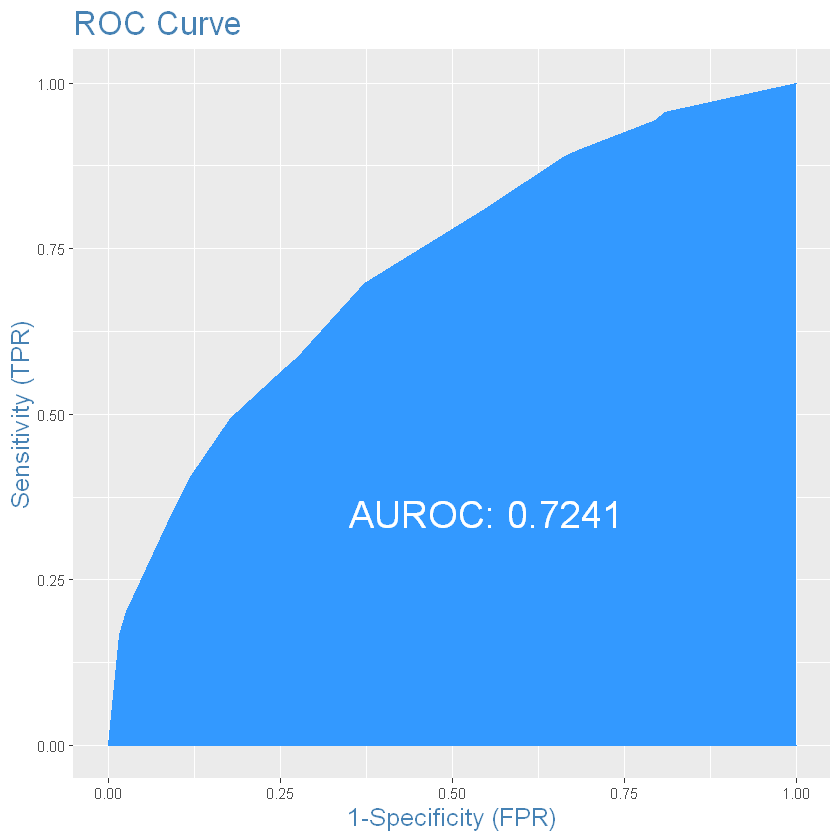
Розділимо результати прогнозування на класи:

test_results$PartyPredicted_Class <- ifelse(test_results$PartyPredicted > optCutOff, 1, 0)

Confusion matrix:

cm <- caret::confusionMatrix(factor(test_results$deposit), 
                             factor(test_results$PartyPredicted_Class), 
                             positive = "1")
cm

Confusion Matrix and Statistics

          Reference
Prediction    0    1
         0 1535  522
         1  803 1046
                                          
               Accuracy : 0.6608          
                 95% CI : (0.6457, 0.6756)
    No Information Rate : 0.5986          
    P-Value [Acc > NIR] : 6.520e-16       
                                          
                  Kappa : 0.3144          
                                          
 Mcnemar's Test P-Value : 1.446e-14       
                                          
            Sensitivity : 0.6671          
            Specificity : 0.6565          
         Pos Pred Value : 0.5657          
         Neg Pred Value : 0.7462          
             Prevalence : 0.4014          
         Detection Rate : 0.2678          
   Detection Prevalence : 0.4734          
      Balanced Accuracy : 0.6618          
                                          
       'Positive' Class : 1               
                                          

Оцінимо збалансовану точність класифікації:

BAcc # value for previous model

0.655537676754586

BAcc1 <- cm$byClass[["Balanced Accuracy"]]
BAcc1

0.661817945741171

---

7.8 Desision Tree with c50

Скористаємося алгоритмом C50 для побудови дерева рішень. Для початку потрібно виіхдний показник перетворити у категоріальний (factor):

# lets make anew temporary dataset for modeling with target output as factor

train_data_tmp <- train_data %>%
    mutate(deposit = factor(train_data$deposit, levels = c(0,1)))

test_data_tmp <- test_data %>%
    mutate(deposit = factor(test_data$deposit, levels = c(0,1)))

Побудуємо модель:

library(C50)
c5_model <- C5.0(deposit ~ ., data = train_data_tmp)

Переглянемо модель:

summary(c5_model)
# its hard to check the nodes

Call:
C5.0.formula(formula = deposit ~ ., data = train_data_tmp)


C5.0 [Release 2.07 GPL Edition]     Mon Oct 03 18:54:18 2022
-------------------------------

Class specified by attribute `outcome'

Read 7256 cases (18 attributes) from undefined.data

Decision tree:

poutcoume_success > 0: 1 (693/56)
poutcoume_success <= 0:
:...pdays > 374: 1 (75/10)
    pdays <= 374:
    :...age > 60: 1 (292/66)
        age <= 60:
        :...contact = unknown:
            :...poutcome = success: 0 (0)
            :   poutcome in {failure,other}: 1 (3)
            :   poutcome = unknown:
            :   :...month in [oct-dec]: 1 (20/2)
            :       month in [jan-sep]:
            :       :...month in [jan-apr]: 1 (10/1)
            :           month in [may-sep]:
            :           :...marital = married: 0 (893/157)
            :               marital in {divorced,single}:
            :               :...default = yes:
            :                   :...marital = divorced: 0 (7/2)
            :                   :   marital = single:
            :                   :   :...day <= 16: 1 (6)
            :                   :       day > 16: 0 (7/2)
            :                   default = no:
            :                   :...day <= 29: 0 (564/139)
            :                       day > 29:
            :                       :...campaign > 7: 1 (4)
            :                           campaign <= 7:
            :                           :...campaign <= 1: 1 (5/1)
            :                               campaign > 1: 0 (19/7)
            contact in {cellular,telephone}:
            :...month = dec: 1 (32/3)
                month in [jan-nov]:
                :...housing = yes:
                    :...month = nov:
                    :   :...day <= 16: 1 (23/7)
                    :   :   day > 16: 0 (264/65)
                    :   month in [jan-oct]:
                    :   :...month in [sep-oct]: 1 (47/7)
                    :       month in [jan-aug]:
                    :       :...contact = telephone: 0 (110/17)
                    :           contact = cellular:
                    :           :...marital in {divorced,
                    :               :           married}: 0 (1115/408)
                    :               marital = single:
                    :               :...pdays_flag > 0:
                    :                   :...education in {primary,
                    :                   :   :             unknown}: 0 (13/3)
                    :                   :   education = secondary:
                    :                   :   :...loan = no: 0 (69/19)
                    :                   :   :   loan = yes: 1 (8/2)
                    :                   :   education = tertiary:
                    :                   :   :...poutcome = failure: 1 (55/24)
                    :                   :       poutcome in {other,success,
                    :                   :                    unknown}: 0 (17/3)
                    :                   pdays_flag <= 0:
                    :                   :...job in {entrepreneur,management,
                    :                       :       retired,
                    :                       :       services}: 0 (129/55)
                    :                       job in {housemaid,self-employed,
                    :                       :       student,unemployed,
                    :                       :       unknown}: 1 (35/13)
                    :                       job = admin.:
                    :                       :...campaign <= 2: 1 (42/20)
                    :                       :   campaign > 2:
                    :                       :   :...loan = no: 0 (12)
                    :                       :       loan = yes: 1 (4/1)
                    :                       job = technician: [S1]
                    :                       job = blue-collar:
                    :                       :...loan = yes: 1 (10)
                    :                           loan = no: [S2]
                    housing = no:
                    :...loan = yes:
                        :...month = jan: 0 (20/1)
                        :   month in [feb-nov]:
                        :   :...age > 37: 0 (170/39)
                        :       age <= 37:
                        :       :...job in {admin.,housemaid,management,
                        :           :       retired,self-employed,student,
                        :           :       unknown}: 0 (58/20)
                        :           job = unemployed: 1 (1)
                        :           job = blue-collar:
                        :           :...education in {primary,
                        :           :   :             tertiary}: 0 (3)
                        :           :   education in {secondary,
                        :           :                 unknown}: 1 (20/5)
                        :           job = entrepreneur:
                        :           :...balance <= 935: 0 (5/1)
                        :           :   balance > 935: 1 (2)
                        :           job = services:
                        :           :...day <= 9: 0 (6)
                        :           :   day > 9: 1 (6/1)
                        :           job = technician:
                        :           :...age <= 29: 1 (11/3)
                        :               age > 29: 0 (16/3)
                        loan = no:
                        :...balance <= 105:
                            :...day <= 5:
                            :   :...month in [jan-feb]: 0 (22/8)
                            :   :   month in [mar-nov]: 1 (28/4)
                            :   day > 5:
                            :   :...month in [jan-apr]:
                            :       :...month in [feb-apr]: 1 (42/10)
                            :       :   month = jan:
                            :       :   :...day <= 20: 1 (4)
                            :       :       day > 20: 0 (32/9)
                            :       month in [may-nov]:
                            :       :...month in [may-aug]: 0 (283/72)
                            :           month in [sep-nov]:
                            :           :...day > 21: 1 (11)
                            :               day <= 21:
                            :               :...balance <= 86: 0 (45/16)
                            :                   balance > 86: 1 (3)
                            balance > 105:
                            :...month in [jan-jun]:
                                :...month in [mar-jun]:
                                :   :...pdays <= 293: 1 (470/88)
                                :   :   pdays > 293:
                                :   :   :...marital = divorced: 1 (4)
                                :   :       marital in {married,
                                :   :                   single}: 0 (20/8)
                                :   month in [jan-feb]:
                                :   :...day > 27: 0 (67/17)
                                :       day <= 27:
                                :       :...day > 9: 1 (71/6)
                                :           day <= 9: [S3]
                                month in [jul-nov]:
                                :...pdays_flag > 0:
                                    :...month in [jul-oct]: 1 (101/15)
                                    :   month = nov:
                                    :   :...campaign > 2: 0 (4)
                                    :       campaign <= 2:
                                    :       :...day <= 17: 1 (20/2)
                                    :           day > 17:
                                    :           :...pdays <= 106: 1 (5/1)
                                    :               pdays > 106: 0 (8)
                                    pdays_flag <= 0:
                                    :...age <= 29: 1 (92/14)
                                        age > 29:
                                        :...marital = divorced:
                                            :...balance > 710: 1 (44/9)
                                            :   balance <= 710: [S4]
                                            marital in {married,single}:
                                            :...campaign <= 1: [S5]
                                                campaign > 1:
                                                :...day <= 10:
                                                    :...campaign > 7: 0 (5)
                                                    :   campaign <= 7: [S6]
                                                    day > 10: [S7]

SubTree [S1]

education in {primary,unknown}: 0 (2)
education = tertiary:
:...month in [jan-jul]: 1 (25/9)
:   month = aug: 0 (4)
education = secondary:
:...month = jan: 0 (3)
    month in [feb-aug]:
    :...month in [feb-apr]: 1 (16/3)
        month in [may-aug]: 0 (25/10)

SubTree [S2]

education = unknown: 0 (0)
education = tertiary: 1 (1)
education = primary:
:...age <= 27: 1 (3)
:   age > 27:
:   :...age <= 46: 0 (13/4)
:       age > 46: 1 (2)
education = secondary:
:...age <= 23: 1 (4)
    age > 23:
    :...month in [jan-may]: 0 (24/5)
        month in [jun-aug]:
        :...day <= 14: 0 (6/2)
            day > 14: 1 (6)

SubTree [S3]

education = unknown: 0 (7/2)
education = primary:
:...marital in {divorced,married}: 0 (10/2)
:   marital = single: 1 (3)
education = tertiary:
:...pdays <= 192: 1 (59/24)
:   pdays > 192: 0 (5)
education = secondary:
:...marital = divorced: 0 (3)
    marital = married:
    :...balance <= 1381: 0 (16/4)
    :   balance > 1381: 1 (8/1)
    marital = single:
    :...day <= 7: 0 (27/5)
        day > 7: 1 (7/1)

SubTree [S4]

job in {admin.,self-employed,unemployed}: 1 (9/1)
job in {blue-collar,entrepreneur,housemaid,management,retired,services,student,
:       unknown}: 0 (19/7)
job = technician:
:...age <= 54: 0 (11/2)
    age > 54: 1 (3)

SubTree [S5]

contact = telephone: 1 (16/1)
contact = cellular:
:...education in {primary,unknown}: 0 (28/8)
    education in {secondary,tertiary}: 1 (136/56)

SubTree [S6]

job in {admin.,retired,self-employed,student}: 1 (12/1)
job in {entrepreneur,housemaid,unemployed,unknown}: 0 (7/1)
job = blue-collar:
:...campaign <= 5: 0 (8/1)
:   campaign > 5: 1 (2)
job = services:
:...balance <= 755: 0 (3)
:   balance > 755: 1 (4)
job = technician:
:...contact = cellular: 1 (19/4)
:   contact = telephone: 0 (2)
job = management:
:...contact = telephone: 1 (2)
    contact = cellular:
    :...age <= 45: 1 (20/7)
        age > 45: 0 (7/1)

SubTree [S7]

job in {admin.,housemaid,management,self-employed,services,student,
:       unknown}: 0 (215/68)
job = unemployed: 1 (10/3)
job = blue-collar:
:...marital = married: 0 (40/16)
:   marital = single: 1 (3)
job = entrepreneur:
:...balance <= 1679: 0 (5)
:   balance > 1679: 1 (4/1)
job = retired:
:...contact = telephone: 1 (3)
:   contact = cellular:
:   :...day <= 16: 1 (5)
:       day > 16:
:       :...age <= 53: 1 (2)
:           age > 53: 0 (12/1)
job = technician:
:...education = primary: 0 (0)
    education = unknown: 1 (1)
    education = tertiary:
    :...age <= 39: 0 (21/6)
    :   age > 39: 1 (7/1)
    education = secondary:
    :...age <= 34: 0 (16)
        age > 34:
        :...marital = married: 0 (30/8)
            marital = single:
            :...day <= 21: 1 (8)
                day > 21: 0 (5/1)


Evaluation on training data (7256 cases):

        Decision Tree   
      ----------------  
      Size      Errors  

       124 1709(23.6%)   <<


       (a)   (b)    <-classified as
      ----  ----
      3332   484    (a): class 0
      1225  2215    (b): class 1


    Attribute usage:

    100.00% poutcoume_success
     90.45% pdays
     89.42% age
     85.39% contact
     85.35% month
     63.75% housing
     54.99% marital
     37.22% loan
     30.71% balance
     30.04% day
     22.19% poutcome
     20.70% pdays_flag
     13.91% job
     10.76% campaign
      9.87% education
      8.43% default


Time: 0.1 secs

Здійснимо прогноз значень:

train_results$C5Predicted <- predict(c5_model, train_data_tmp)
test_results$C5Predicted <- predict(c5_model, test_data_tmp)

ROC-крива та AUROC:

plotROC(as.numeric(test_results$deposit), as.numeric(test_results$C5Predicted))
# you can see that current algorithm is not very good for this data, partykit is much better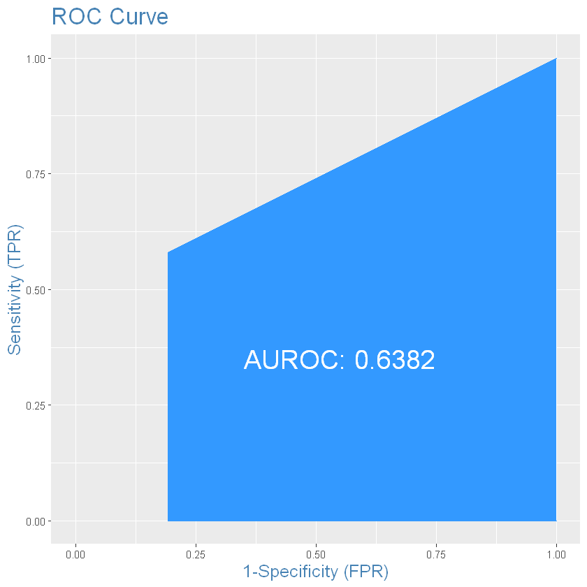

Confusion Matrix:

cm <- caret::confusionMatrix(factor(test_results$deposit), 
                             test_results$C5Predicted, 
                             positive = "1")
cm

Confusion Matrix and Statistics

          Reference
Prediction    0    1
         0 1662  395
         1  777 1072
                                          
               Accuracy : 0.6999          
                 95% CI : (0.6853, 0.7143)
    No Information Rate : 0.6244          
    P-Value [Acc > NIR] : < 2.2e-16       
                                          
                  Kappa : 0.3918          
                                          
 Mcnemar's Test P-Value : < 2.2e-16       
                                          
            Sensitivity : 0.7307          
            Specificity : 0.6814          
         Pos Pred Value : 0.5798          
         Neg Pred Value : 0.8080          
             Prevalence : 0.3756          
         Detection Rate : 0.2744          
   Detection Prevalence : 0.4734          
      Balanced Accuracy : 0.7061          
                                          
       'Positive' Class : 1               
                                          

Збалансована точність моделі:

BAcc # rpart
BAcc1 # partykit

0.655537676754586

0.661817945741171

BAcc2 <- cm$byClass[["Balanced Accuracy"]]
BAcc2
# but balanced accuracy is the best. So this model better classify both good and bad events

0.706084913609872

---

7.9 RandomForest

You can use random forest with default or special training parameters.

head(train_results)

A data.frame: 6 × 5

	No	deposit	RPartPredicted	PartyPredicted	C5Predicted
	<int>	<dbl>	<dbl>	<dbl>	<fct>
3	1	1	0.2287751	0.1827243	0
5	2	1	0.2287751	0.1827243	0
6	3	1	0.2287751	0.2746365	0
11	4	1	0.2287751	0.2746365	0
12	5	1	0.2287751	0.1827243	0
14	6	1	0.2287751	0.2746365	0

head(train_data)

A data.frame: 6 × 18

	age	job	marital	education	default	balance	housing	loan	contact	day	month	campaign	pdays	previous	poutcome	deposit	pdays_flag	poutcoume_success
	<int>	<fct>	<fct>	<fct>	<fct>	<int>	<fct>	<fct>	<fct>	<int>	<ord>	<int>	<int>	<int>	<fct>	<dbl>	<dbl>	<dbl>
3	41	technician	married	secondary	no	1270	yes	no	unknown	5	may	1	-1	0	unknown	1	0	0
5	54	admin.	married	tertiary	no	184	no	no	unknown	5	may	2	-1	0	unknown	1	0	0
6	42	management	single	tertiary	no	0	yes	yes	unknown	5	may	2	-1	0	unknown	1	0	0
11	38	admin.	single	secondary	no	100	yes	no	unknown	7	may	1	-1	0	unknown	1	0	0
12	30	blue-collar	married	secondary	no	309	yes	no	unknown	7	may	2	-1	0	unknown	1	0	0
14	46	blue-collar	single	tertiary	no	460	yes	no	unknown	7	may	2	-1	0	unknown	1	0	0

#install.packages("randomForest")

table(train_data$deposit)

   0    1 
3816 3440 

suppressMessages(library(randomForest))

rf_model <- randomForest(deposit ~ ., 
                         data=train_data, 
                         ntree=200, 
                         mtry=2, 
                         importance=TRUE) #Should importance of predictors be assessed?

Warning message in randomForest.default(m, y, ...):
"The response has five or fewer unique values.  Are you sure you want to do regression?"

ntree - Number of trees to grow. This should not be set to too small a number, to ensure that every input row gets predicted at least a few times.

mtry - Number of variables randomly sampled as candidates at each split.

rf_model

Call:
 randomForest(formula = deposit ~ ., data = train_data, ntree = 200,      mtry = 2, importance = TRUE) 
               Type of random forest: regression
                     Number of trees: 200
No. of variables tried at each split: 2

          Mean of squared residuals: 0.1909128
                    % Var explained: 23.43

Можемо провести аналіз важливості параметрів у залежності від критерію зменшення точності або зменшення джині:

varImpPlot(rf_model)

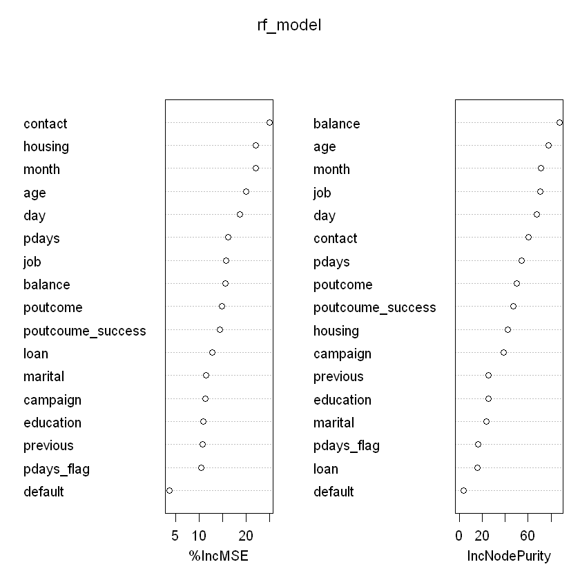
• MeanDecreaseAccuracy: gives a rough estimate of the loss in prediction performance when that particular variable is omitted from the training set. Caveat: if two variables are somewhat redundant, then omitting one of them may not lead to massive gains in prediction performance, but would make the second variable more important.

• MeanDecreaseGini: GINI is a measure of node impurity. Think of it like this, if you use this feature to split the data, how pure will the nodes be? Highest purity means that each node contains only elements of a single class. Assessing the decrease in GINI when that feature is omitted leads to an understanding of how important that feature is to split the data correctly.

train_results$RF <- predict(rf_model, train_data)
test_results$RF <- predict(rf_model, test_data)

optCutOff <- optimalCutoff(train_results$deposit, train_results$RF)
optCutOff

0.426968327910145

test_results$RF_Class = ifelse(test_results$RF > optCutOff, 1, 0)

ROC-крива та AUROC:

plotROC(as.numeric(test_results$deposit), as.numeric(test_results$RF))

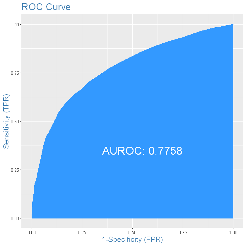
# Balanced accuracy is much better the before!
cm <- caret::confusionMatrix(factor(test_results$deposit), 
                             factor(test_results$RF_Class), 
                             positive = "1")
cm

Confusion Matrix and Statistics

          Reference
Prediction    0    1
         0 1411  646
         1  506 1343
                                          
               Accuracy : 0.7051          
                 95% CI : (0.6905, 0.7193)
    No Information Rate : 0.5092          
    P-Value [Acc > NIR] : < 2.2e-16       
                                          
                  Kappa : 0.4107          
                                          
 Mcnemar's Test P-Value : 4.216e-05       
                                          
            Sensitivity : 0.6752          
            Specificity : 0.7360          
         Pos Pred Value : 0.7263          
         Neg Pred Value : 0.6860          
             Prevalence : 0.5092          
         Detection Rate : 0.3438          
   Detection Prevalence : 0.4734          
      Balanced Accuracy : 0.7056          
                                          
       'Positive' Class : 1               
                                          

Balanced accuracy is hte best for now

---

7.10 xgBoost

Our next step is testing gradient boosting with xgboost algorithm.

suppressMessages(library(xgboost))

For complex algorithm like random forest or xgboost model training is the most important stage.

XGBoost only works with numeric vectors. Therefore, you need to convert all other forms of data into numeric vectors.

train_labels <- train_data$deposit
test_labels <- test_data$deposit

xgb_train_data <- xgb.DMatrix(data = model.matrix(deposit~., data = train_data),
                              label = train_labels)
xgb_test_data <- xgb.DMatrix(data = model.matrix(deposit~., data = test_data),
                              label = test_labels)
xgb_test_data

xgb.DMatrix  dim: 3906 x 44  info: label  colnames: yes

We will train decision tree model using the following parameters:

• objective = "binary:logistic": we will train a binary classification model ;
• max.depth = 2: the trees won’t be deep, because our case is very simple ;
• nthread = 2: the number of CPU threads we are going to use;
• nrounds = 2: there will be two passes on the data, the second one will enhance the model by further reducing the difference between ground truth and prediction.

xgb_model <- xgboost(data = xgb_train_data, 
                     label = train_labels, 
                     max.depth = 2, 
                     #eta = 1, 
                     nthread = 2, 
                     nrounds = 2, 
                     objective = "binary:logistic")
xgb_model

Warning message in xgb.get.DMatrix(data, label, missing, weight, nthread = merged$nthread):
"xgboost: label will be ignored."

[1] train-logloss:0.659975 
[2] train-logloss:0.635883 

##### xgb.Booster
raw: 5.8 Kb 
call:
  xgb.train(params = params, data = dtrain, nrounds = nrounds, 
    watchlist = watchlist, verbose = verbose, print_every_n = print_every_n, 
    early_stopping_rounds = early_stopping_rounds, maximize = maximize, 
    save_period = save_period, save_name = save_name, xgb_model = xgb_model, 
    callbacks = callbacks, max.depth = 2, nthread = 2, objective = "binary:logistic")
params (as set within xgb.train):
  max_depth = "2", nthread = "2", objective = "binary:logistic", validate_parameters = "TRUE"
xgb.attributes:
  niter
callbacks:
  cb.print.evaluation(period = print_every_n)
  cb.evaluation.log()
# of features: 44 
niter: 2
nfeatures : 44 
evaluation_log:
 iter train_logloss
    1     0.6599753
    2     0.6358826

# predict data
train_results$XGB <- predict(xgb_model, xgb_train_data)
test_results$XGB <- predict(xgb_model, xgb_test_data)

head(test_results)

A data.frame: 6 × 10

	No	deposit	RPartPredicted	RPartPredicted_Class	PartyPredicted	PartyPredicted_Class	C5Predicted	RF	RF_Class	XGB
	<int>	<dbl>	<dbl>	<dbl>	<dbl>	<dbl>	<fct>	<dbl>	<dbl>	<dbl>
1	1	1	0.2287751	0	0.1827243	0	0	0.2377513	0	0.3903929
2	2	1	0.2287751	0	0.1827243	0	0	0.2456910	0	0.3903929
4	3	1	0.2287751	0	0.1827243	0	0	0.2173557	0	0.3903929
7	4	1	0.2287751	0	0.1827243	0	0	0.2370295	0	0.3903929
8	5	1	0.2287751	0	0.2746365	0	0	0.3459498	0	0.3903929
9	6	1	0.2287751	0	0.1827243	0	0	0.1872509	0	0.3903929

Optimal cutoff:

optCutOff <- optimalCutoff(train_results$deposit, train_results$XGB)
optCutOff

0.473113248348236

# evaluate classification class
test_results$XGB_Class = ifelse(test_results$XGB > optCutOff, 1, 0)

plotROC(as.numeric(test_results$deposit), as.numeric(test_results$XGB))

# Balanced accuracy is not better, random forest wins for now!
cm <- caret::confusionMatrix(factor(test_results$deposit), 
                             factor(test_results$XGB_Class), 
                             positive = "1")
cm

Confusion Matrix and Statistics

          Reference
Prediction    0    1
         0 1777  280
         1 1065  784
                                          
               Accuracy : 0.6557          
                 95% CI : (0.6405, 0.6706)
    No Information Rate : 0.7276          
    P-Value [Acc > NIR] : 1               
                                          
                  Kappa : 0.2942          
                                          
 Mcnemar's Test P-Value : <2e-16          
                                          
            Sensitivity : 0.7368          
            Specificity : 0.6253          
         Pos Pred Value : 0.4240          
         Neg Pred Value : 0.8639          
             Prevalence : 0.2724          
         Detection Rate : 0.2007          
   Detection Prevalence : 0.4734          
      Balanced Accuracy : 0.6811          
                                          
       'Positive' Class : 1               
                                          

---

7.11 lightgbm

Light gbm is one of most useful package for machine learning. It has one super power: speed of calculations. While you using very big datasets randomForest and xgBoost work slow, but lightgbm works better.

For this algorithm we should convert our data to special matrices too. So, lets install packages for example:

# ALERT sometimes you need to unistall Matrix in RSTudio and install it again
suppressMessages(library(Matrix))                      
suppressMessages(library(lightgbm))

Lets use binning technique for data preprocessing

suppressMessages(library(scorecard))

vars_list <- train_data %>%
  select(-deposit) %>%
  names()
vars_list

1. 'age'
2. 'job'
3. 'marital'
4. 'education'
5. 'default'
6. 'balance'
7. 'housing'
8. 'loan'
9. 'contact'
10. 'day'
11. 'month'
12. 'campaign'
13. 'pdays'
14. 'previous'
15. 'poutcome'
16. 'pdays_flag'
17. 'poutcoume_success'

bin_class <- woebin(train_data, 
                    y = "deposit", 
                    x = vars_list, 
                    positive = 1, # the value in deposit that indicates event                   
                    bin_num_limit = 20)
# bin_class - to check bins

[INFO] creating woe binning ... 

train_woe <- woebin_ply(train_data, bin_class)
test_woe <- woebin_ply(test_data, bin_class)
head(train_woe)

[INFO] converting into woe values ... 
[INFO] converting into woe values ... 

A data.table: 6 × 18

deposit	age_woe	job_woe	marital_woe	education_woe	default_woe	balance_woe	housing_woe	loan_woe	contact_woe	day_woe	month_woe	campaign_woe	pdays_woe	previous_woe	poutcome_woe	pdays_flag_woe	poutcoume_success_woe
<dbl>	<dbl>	<dbl>	<dbl>	<dbl>	<dbl>	<dbl>	<dbl>	<dbl>	<dbl>	<dbl>	<dbl>	<dbl>	<dbl>	<dbl>	<dbl>	<dbl>	<dbl>
1	-0.1919797	0.18206313	-0.1591497	-0.1114005	0	0.34944916	-0.4636881	0.08789815	-1.11036	-0.2931007	-0.6621753	0.22554244	-0.2605003	-0.2597224	-0.2592721	-0.2597224	-0.1899974
1	-0.1919797	-0.02410209	-0.1591497	0.2697353	0	-0.34928490	0.4042223	0.08789815	-1.11036	-0.2931007	-0.6621753	-0.03160046	-0.2605003	-0.2597224	-0.2592721	-0.2597224	-0.1899974
1	-0.1919797	0.17010635	0.2785068	0.2697353	0	-0.34928490	-0.4636881	-0.61989139	-1.11036	-0.2931007	-0.6621753	-0.03160046	-0.2605003	-0.2597224	-0.2592721	-0.2597224	-0.1899974
1	-0.1919797	-0.02410209	0.2785068	-0.1114005	0	-0.34928490	-0.4636881	0.08789815	-1.11036	-0.2931007	-0.6621753	0.22554244	-0.2605003	-0.2597224	-0.2592721	-0.2597224	-0.1899974
1	-0.1919797	-0.47176755	-0.1591497	-0.1114005	0	-0.05026394	-0.4636881	0.08789815	-1.11036	-0.2931007	-0.6621753	-0.03160046	-0.2605003	-0.2597224	-0.2592721	-0.2597224	-0.1899974
1	-0.1919797	-0.47176755	0.2785068	0.2697353	0	-0.05026394	-0.4636881	0.08789815	-1.11036	-0.2931007	-0.6621753	-0.03160046	-0.2605003	-0.2597224	-0.2592721	-0.2597224	-0.1899974

vars_list <- train_woe %>%
  select(-deposit) %>%
  names() 
vars_list

1. 'age_woe'
2. 'job_woe'
3. 'marital_woe'
4. 'education_woe'
5. 'default_woe'
6. 'balance_woe'
7. 'housing_woe'
8. 'loan_woe'
9. 'contact_woe'
10. 'day_woe'
11. 'month_woe'
12. 'campaign_woe'
13. 'pdays_woe'
14. 'previous_woe'
15. 'poutcome_woe'
16. 'pdays_flag_woe'
17. 'poutcoume_success_woe'

head(test_woe %>% select(vars_list))

Note: Using an external vector in selections is ambiguous.
i Use `all_of(vars_list)` instead of `vars_list` to silence this message.
i See <https://tidyselect.r-lib.org/reference/faq-external-vector.html>.
This message is displayed once per session.

A data.table: 6 × 17

age_woe	job_woe	marital_woe	education_woe	default_woe	balance_woe	housing_woe	loan_woe	contact_woe	day_woe	month_woe	campaign_woe	pdays_woe	previous_woe	poutcome_woe	pdays_flag_woe	poutcoume_success_woe
<dbl>	<dbl>	<dbl>	<dbl>	<dbl>	<dbl>	<dbl>	<dbl>	<dbl>	<dbl>	<dbl>	<dbl>	<dbl>	<dbl>	<dbl>	<dbl>	<dbl>
-0.1919797	-0.02410209	-0.15914969	-0.1114005	0	0.34944916	-0.4636881	0.08789815	-1.11036	-0.2931007	-0.6621753	0.2255424	-0.2605003	-0.2597224	-0.2592721	-0.2597224	-0.1899974
-0.1919797	-0.02410209	-0.15914969	-0.1114005	0	-0.34928490	0.4042223	0.08789815	-1.11036	-0.2931007	-0.6621753	0.2255424	-0.2605003	-0.2597224	-0.2592721	-0.2597224	-0.1899974
-0.1919797	-0.26465641	-0.15914969	-0.1114005	0	0.34944916	-0.4636881	0.08789815	-1.11036	-0.2931007	-0.6621753	0.2255424	-0.2605003	-0.2597224	-0.2592721	-0.2597224	-0.1899974
-0.1919797	0.17010635	-0.15914969	0.2697353	0	0.34944916	-0.4636881	-0.61989139	-1.11036	-0.2931007	-0.6621753	0.2255424	-0.2605003	-0.2597224	-0.2592721	-0.2597224	-0.1899974
1.2441251	0.73838226	0.01571154	-0.1114005	0	-0.05026394	-0.4636881	0.08789815	-1.11036	-0.2931007	-0.6621753	0.2255424	-0.2605003	-0.2597224	-0.2592721	-0.2597224	-0.1899974
-0.1919797	0.18206313	-0.15914969	-0.1114005	0	-0.34928490	-0.4636881	0.08789815	-1.11036	-0.2931007	-0.6621753	0.2255424	-0.2605003	-0.2597224	-0.2592721	-0.2597224	-0.1899974

train_sparse = Matrix(as.matrix(train_woe %>% select(vars_list)), sparse=TRUE)
test_sparse = Matrix(as.matrix(test_woe %>% select(vars_list)), sparse=TRUE)

lgb.train = lgb.Dataset(data = train_sparse, label = train_woe$deposit, free_raw_data = FALSE)
lgb.test = lgb.Dataset(data = test_sparse, label = test_woe$deposit, free_raw_data = FALSE)

lgb.grid = list(objective = "binary",
                metric = "auc",
                #save_binary = T,
                max_bin = 32,
                num_leaves = 33)

lgb.train.cv = lgb.train(params = lgb.grid,
                         data = lgb.train,                         
                         nrounds = 15,                         
                         early_stopping_round = 300,
                         #categorical_feature = categoricals.vec,
                         valids = list(test = lgb.test),
                         verbose = 1) 

[LightGBM] [Info] Number of positive: 3440, number of negative: 3816
[LightGBM] [Warning] Auto-choosing row-wise multi-threading, the overhead of testing was 0.020781 seconds.
You can set `force_row_wise=true` to remove the overhead.
And if memory is not enough, you can set `force_col_wise=true`.
[LightGBM] [Info] Total Bins 74
[LightGBM] [Info] Number of data points in the train set: 7256, number of used features: 16
[LightGBM] [Info] [binary:BoostFromScore]: pavg=0.474090 -> initscore=-0.103731
[LightGBM] [Info] Start training from score -0.103731
[1] "[1]:  test's auc:0.759236"
[1] "[2]:  test's auc:0.760231"
[1] "[3]:  test's auc:0.763489"
[1] "[4]:  test's auc:0.763607"
[1] "[5]:  test's auc:0.763681"
[1] "[6]:  test's auc:0.763814"
[1] "[7]:  test's auc:0.762936"
[1] "[8]:  test's auc:0.765679"
[1] "[9]:  test's auc:0.766939"
[1] "[10]:  test's auc:0.767712"
[1] "[11]:  test's auc:0.768105"
[1] "[12]:  test's auc:0.768932"
[1] "[13]:  test's auc:0.769262"
[1] "[14]:  test's auc:0.769862"
[1] "[15]:  test's auc:0.770532"

# predict data
train_results$LGBM <- predict(lgb.train.cv, train_sparse)
test_results$LGBM <- predict(lgb.train.cv, test_sparse)

head(test_results)

A data.frame: 6 × 12

	No	deposit	RPartPredicted	RPartPredicted_Class	PartyPredicted	PartyPredicted_Class	C5Predicted	RF	RF_Class	XGB	XGB_Class	LGBM
	<int>	<dbl>	<dbl>	<dbl>	<dbl>	<dbl>	<fct>	<dbl>	<dbl>	<dbl>	<dbl>	<dbl>
1	1	1	0.2287751	0	0.1827243	0	0	0.2377513	0	0.3903929	0	0.2076138
2	2	1	0.2287751	0	0.1827243	0	0	0.2456910	0	0.3903929	0	0.1978679
4	3	1	0.2287751	0	0.1827243	0	0	0.2173557	0	0.3903929	0	0.2076138
7	4	1	0.2287751	0	0.1827243	0	0	0.2370295	0	0.3903929	0	0.2076138
8	5	1	0.2287751	0	0.2746365	0	0	0.3459498	0	0.3903929	0	0.2508506
9	6	1	0.2287751	0	0.1827243	0	0	0.1872509	0	0.3903929	0	0.1978679

# Optimal cutoff:

optCutOff <- optimalCutoff(train_results$deposit, train_results$LGBM)
optCutOff

0.489317324236863

# evaluate classification class
test_results$LGBM_Class = ifelse(test_results$LGBM > optCutOff, 1, 0)
plotROC(as.numeric(test_results$deposit), as.numeric(test_results$LGBM))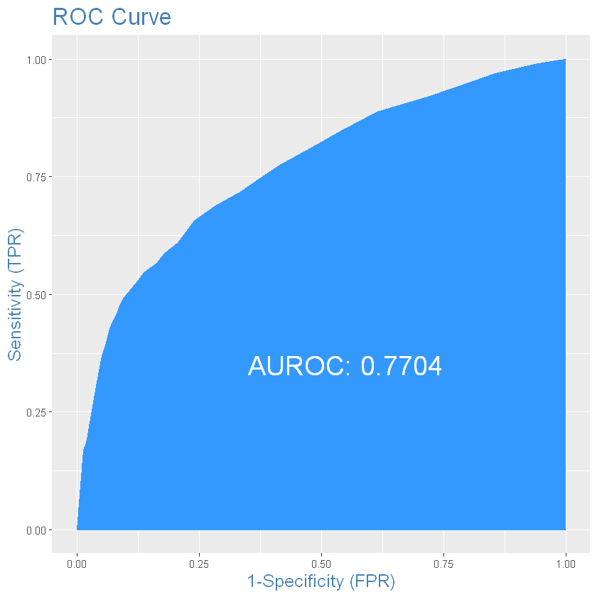

# Balanced accuracy is not better, random forest wins for now!
cm <- caret::confusionMatrix(factor(test_results$deposit), 
                             factor(test_results$LGBM_Class), 
                             positive = "1")
cm

Confusion Matrix and Statistics

          Reference
Prediction    0    1
         0 1667  390
         1  741 1108
                                          
               Accuracy : 0.7104          
                 95% CI : (0.6959, 0.7246)
    No Information Rate : 0.6165          
    P-Value [Acc > NIR] : < 2.2e-16       
                                          
                  Kappa : 0.4136          
                                          
 Mcnemar's Test P-Value : < 2.2e-16       
                                          
            Sensitivity : 0.7397          
            Specificity : 0.6923          
         Pos Pred Value : 0.5992          
         Neg Pred Value : 0.8104          
             Prevalence : 0.3835          
         Detection Rate : 0.2837          
   Detection Prevalence : 0.4734          
      Balanced Accuracy : 0.7160          
                                          
       'Positive' Class : 1               
                                          

---