3  Лінійна регресія. Прокат велосипедів

Курс: “Математичне моделювання в R”

---

Перевірити матеріали лекції!!!

Розділ про прогноз з кроком 10-30. Втрачено окремі комірки коду.

# install.packages("mice")

3.1 Dataset overview

Source: https://www.kaggle.com/c/bike-sharing-demand/data

Dataset description:

You are provided hourly rental data spanning two years. For this competition, the training set is comprised of the first 19 days of each month, while the test set is the 20th to the end of the month. You must predict the total count of bikes rented during each hour covered by the test set, using only information available prior to the rental period.

Data Fields:

• datetime - hourly date + timestamp
• season -
  • 1 = spring
  • 2 = summer
  • 3 = fall
  • 4 = winter
• holiday - whether the day is considered a holiday
• workingday - whether the day is neither a weekend nor holiday
• weather
  • 1: Clear, Few clouds, Partly cloudy, Partly cloudy
  • 2: Mist + Cloudy, Mist + Broken clouds, Mist + Few clouds, Mist
  • 3: Light Snow, Light Rain + Thunderstorm + Scattered clouds, Light Rain + Scattered clouds
  • 4: Heavy Rain + Ice Pallets + Thunderstorm + Mist, Snow + Fog
• temp - temperature in Celsius
• atemp - “feels like” temperature in Celsius
• humidity - relative humidity
• windspeed - wind speed
• casual - number of non-registered user rentals initiated
• registered - number of registered user rentals initiated
• count - number of total rentals (It is target variable. We will predict it!)

data <- read.csv("data/bikes.csv")
head(data)

A data.frame: 6 × 12

	datetime	season	holiday	workingday	weather	temp	atemp	humidity	windspeed	casual	registered	count
	<chr>	<int>	<int>	<int>	<int>	<dbl>	<dbl>	<int>	<dbl>	<int>	<int>	<int>
1	2011-01-01 00:00:00	1	0	0	1	9.84	14.395	81	0.0000	3	13	16
2	2011-01-01 01:00:00	1	0	0	1	9.02	13.635	80	0.0000	8	32	40
3	2011-01-01 02:00:00	1	0	0	1	9.02	13.635	80	0.0000	5	27	32
4	2011-01-01 03:00:00	1	0	0	1	9.84	14.395	75	0.0000	3	10	13
5	2011-01-01 04:00:00	1	0	0	1	9.84	14.395	75	0.0000	0	1	1
6	2011-01-01 05:00:00	1	0	0	2	9.84	12.880	75	6.0032	0	1	1

Описова статистика факторів:

summary(data)

   datetime             season         holiday          workingday    
 Length:10886       Min.   :1.000   Min.   :0.00000   Min.   :0.0000  
 Class :character   1st Qu.:2.000   1st Qu.:0.00000   1st Qu.:0.0000  
 Mode  :character   Median :3.000   Median :0.00000   Median :1.0000  
                    Mean   :2.507   Mean   :0.02857   Mean   :0.6809  
                    3rd Qu.:4.000   3rd Qu.:0.00000   3rd Qu.:1.0000  
                    Max.   :4.000   Max.   :1.00000   Max.   :1.0000  
    weather           temp           atemp          humidity     
 Min.   :1.000   Min.   : 0.82   Min.   : 0.76   Min.   :  0.00  
 1st Qu.:1.000   1st Qu.:13.94   1st Qu.:16.66   1st Qu.: 47.00  
 Median :1.000   Median :20.50   Median :24.24   Median : 62.00  
 Mean   :1.418   Mean   :20.23   Mean   :23.66   Mean   : 61.89  
 3rd Qu.:2.000   3rd Qu.:26.24   3rd Qu.:31.06   3rd Qu.: 77.00  
 Max.   :4.000   Max.   :41.00   Max.   :45.45   Max.   :100.00  
   windspeed          casual         registered        count      
 Min.   : 0.000   Min.   :  0.00   Min.   :  0.0   Min.   :  1.0  
 1st Qu.: 7.002   1st Qu.:  4.00   1st Qu.: 36.0   1st Qu.: 42.0  
 Median :12.998   Median : 17.00   Median :118.0   Median :145.0  
 Mean   :12.799   Mean   : 36.02   Mean   :155.6   Mean   :191.6  
 3rd Qu.:16.998   3rd Qu.: 49.00   3rd Qu.:222.0   3rd Qu.:284.0  
 Max.   :56.997   Max.   :367.00   Max.   :886.0   Max.   :977.0  

3.2 Minimal data preprocessing

Перевіримо вибірку на наявність пропусків за допомогою функції md.pattern() з пакету mice:

anyNA(data)

FALSE

suppressMessages(library(mice))
md.pattern(data, F)

 /\     /\
{  `---'  }
{  O   O  }
==>  V <==  No need for mice. This data set is completely observed.
 \  \|/  /
  `-----'

A matrix: 2 × 13 of type dbl

	datetime	season	holiday	workingday	weather	temp	atemp	humidity	windspeed	casual	registered	count
10886	1	1	1	1	1	1	1	1	1	1	1	1	0
	0	0	0	0	0	0	0	0	0	0	0	0	0

There are no missing data! Great for us!

Перетворимо категоріальні змінні до факторів:

data$season <- factor(data$season)
data$holiday <- factor(data$holiday)
data$workingday <- factor(data$workingday)
data$weather <- factor(data$weather)
data$holiday <- factor(data$holiday)

head(data) # preview data

A data.frame: 6 × 12

	datetime	season	holiday	workingday	weather	temp	atemp	humidity	windspeed	casual	registered	count
	<chr>	<fct>	<fct>	<fct>	<fct>	<dbl>	<dbl>	<int>	<dbl>	<int>	<int>	<int>
1	2011-01-01 00:00:00	1	0	0	1	9.84	14.395	81	0.0000	3	13	16
2	2011-01-01 01:00:00	1	0	0	1	9.02	13.635	80	0.0000	8	32	40
3	2011-01-01 02:00:00	1	0	0	1	9.02	13.635	80	0.0000	5	27	32
4	2011-01-01 03:00:00	1	0	0	1	9.84	14.395	75	0.0000	3	10	13
5	2011-01-01 04:00:00	1	0	0	1	9.84	14.395	75	0.0000	0	1	1
6	2011-01-01 05:00:00	1	0	0	2	9.84	12.880	75	6.0032	0	1	1

У наборі даних наявні 3 вихідних параметра: casual,registered,count, де $casual + registered = count$. Здійснимо прогнозcount`. Видалимо змінні, які використовуватися нами не будуть:

#data$casual <- NULL
#data$registered <- NULL

# or with dplyr
suppressMessages(library(dplyr))
data <- data %>% select(-c(casual, registered))

head(data)

A data.frame: 6 × 10

	datetime	season	holiday	workingday	weather	temp	atemp	humidity	windspeed	count
	<chr>	<fct>	<fct>	<fct>	<fct>	<dbl>	<dbl>	<int>	<dbl>	<int>
1	2011-01-01 00:00:00	1	0	0	1	9.84	14.395	81	0.0000	16
2	2011-01-01 01:00:00	1	0	0	1	9.02	13.635	80	0.0000	40
3	2011-01-01 02:00:00	1	0	0	1	9.02	13.635	80	0.0000	32
4	2011-01-01 03:00:00	1	0	0	1	9.84	14.395	75	0.0000	13
5	2011-01-01 04:00:00	1	0	0	1	9.84	14.395	75	0.0000	1
6	2011-01-01 05:00:00	1	0	0	2	9.84	12.880	75	6.0032	1

3.3 Exploratory data analysis

Оцінимо звязки між числовими змінними та вихідним показником через кореляцію:

data %>%
 select(temp:count) %>% 
 cor() %>%
 as.data.frame()

A data.frame: 5 × 5

	temp	atemp	humidity	windspeed	count
	<dbl>	<dbl>	<dbl>	<dbl>	<dbl>
temp	1.00000000	0.98494811	-0.06494877	-0.01785201	0.3944536
atemp	0.98494811	1.00000000	-0.04353571	-0.05747300	0.3897844
humidity	-0.06494877	-0.04353571	1.00000000	-0.31860699	-0.3173715
windspeed	-0.01785201	-0.05747300	-0.31860699	1.00000000	0.1013695
count	0.39445364	0.38978444	-0.31737148	0.10136947	1.0000000

Щоб оглянути інформацію про частоту спостежень по сезонах варто скористатися записом:

data %>%
 group_by(season) %>%
 summarize(n = n())

A tibble: 4 × 2

season	n
<fct>	<int>
1	2686
2	2733
3	2733
4	2734

library(ggplot2)
# llok like we have almost the same count by each season
ggplot(data, aes(season)) + 
    geom_bar(aes(fill = season)) + 
    theme_bw()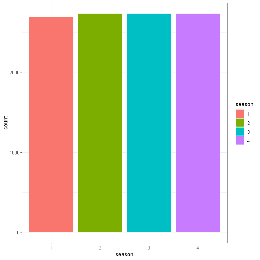

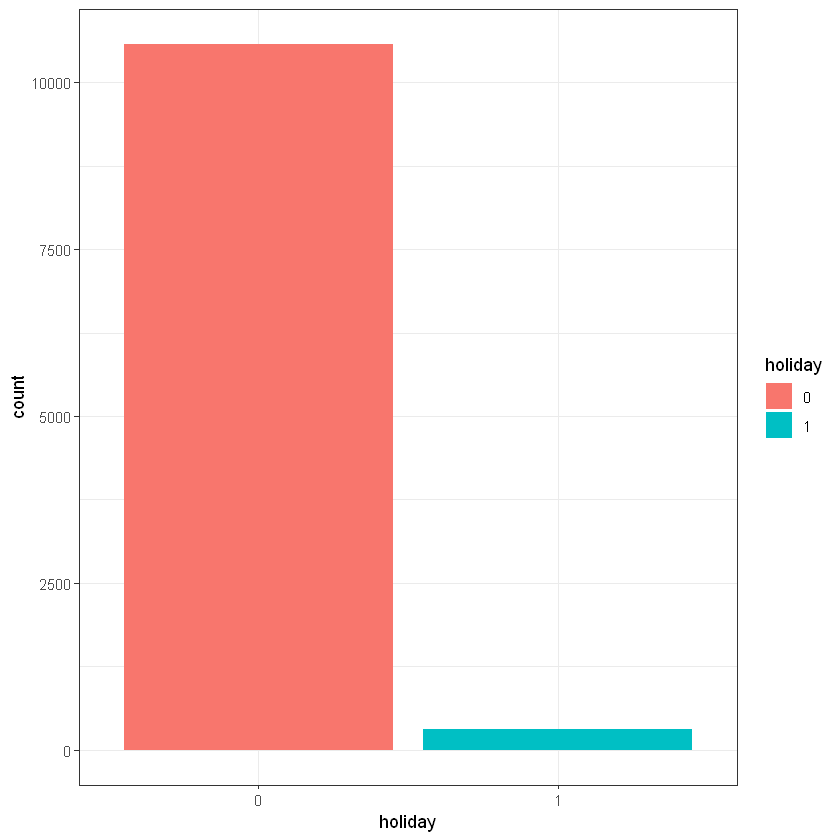
# Holidays plot
data %>%
 group_by(holiday) %>%
 summarize(n = n())

ggplot(data, aes(holiday)) + geom_bar(aes(fill = holiday)) + theme_bw()

A tibble: 2 × 2

holiday	n
<fct>	<int>
0	10575
1	311

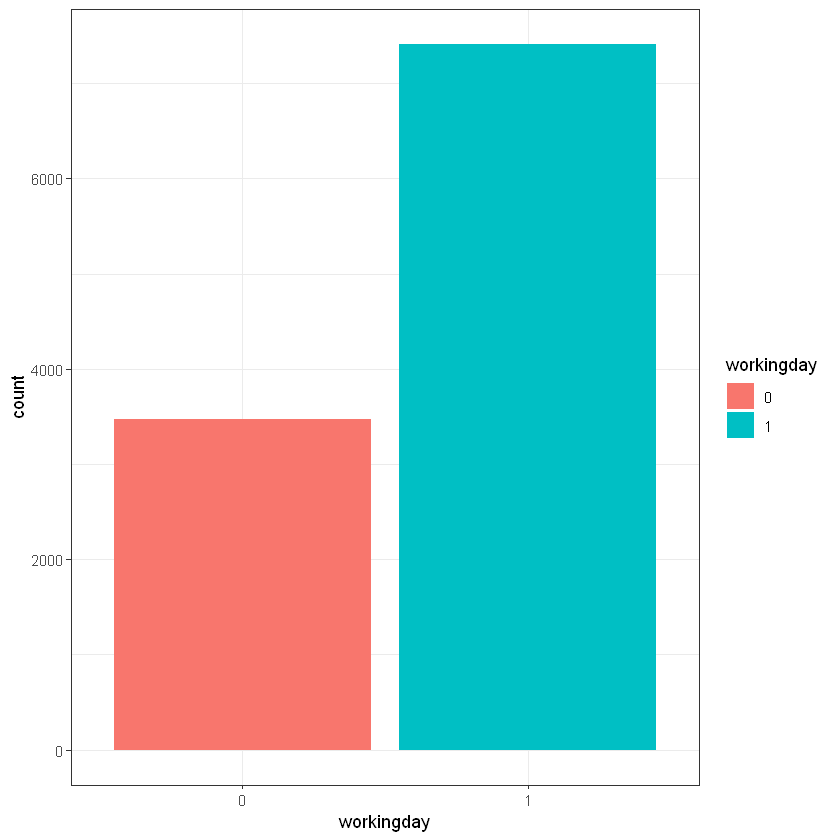
data %>%
 group_by(workingday) %>%
 summarize(n = n())

# Working dats plot
ggplot(data, aes(workingday)) + geom_bar(aes(fill = workingday)) + theme_bw()

A tibble: 2 × 2

workingday	n
<fct>	<int>
0	3474
1	7412

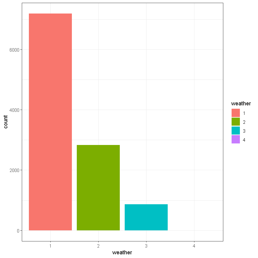
• weather
  • 1: Clear, Few clouds, Partly cloudy, Partly cloudy
  • 2: Mist + Cloudy, Mist + Broken clouds, Mist + Few clouds, Mist
  • 3: Light Snow, Light Rain + Thunderstorm + Scattered clouds, Light Rain + Scattered clouds
  • 4: Heavy Rain + Ice Pallets + Thunderstorm + Mist, Snow + Fog

# weather plot
ggplot(data, aes(weather)) + geom_bar(aes(fill = weather)) + theme_bw()

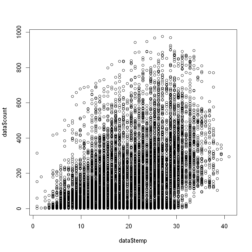
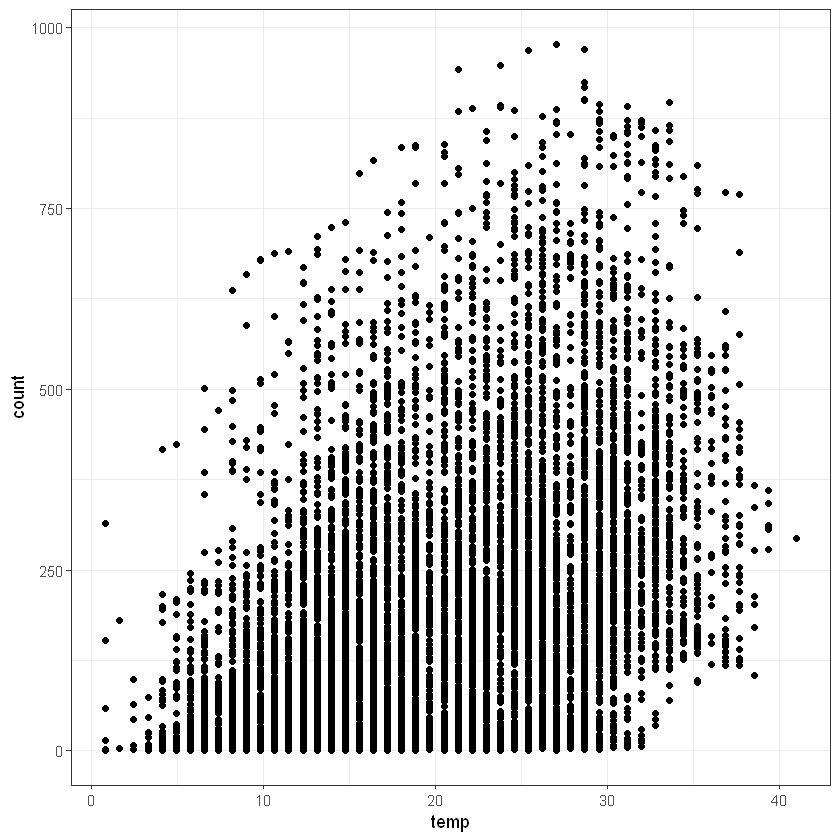
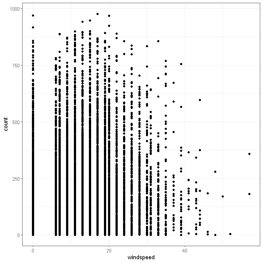
Переглянемо також залежність між числовими факторами та кількістю прокатів байків. Для температури це матиме запис:

# temp
plot(x=data$temp, y=data$count)

ggplot(data, aes(temp, count)) + geom_point() + theme_bw()

# atemp
ggplot(data, aes(atemp, count)) + geom_point() + theme_bw()

# humidity
ggplot(data, aes(humidity, count)) + geom_point() + theme_bw()

# windspeed
ggplot(data, aes(windspeed, count)) + geom_point() + theme_bw()

Переглянемо також загальний розподіл частоти замовлень байків на гістограмі:

ggplot(data, aes(count)) + geom_histogram(bins = 25, alpha = 0.5, fill = 'blue', color='black')  + theme_bw()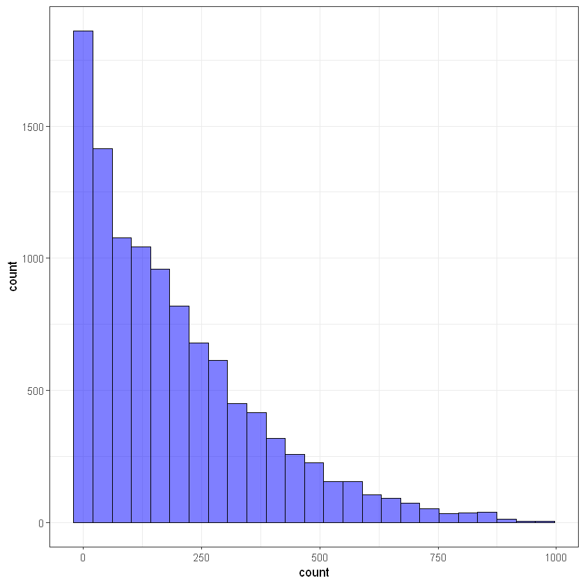

При спробі побудувати графік залежності між датою та кількістю замовлень байків ми отримаємо помилку або графік, що не відповідає порядку дат, оскільки на даний момент R не сприймає поле datetime як дату. Перетворимо дату за допомгою функції as.POSIXct():

data$datetime <- as.POSIXct(data$datetime)
ggplot(data, aes(datetime, count)) + geom_point() + theme_bw()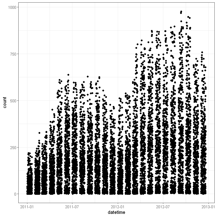

Чи можна прослідкувати зміну кількості замовлень в залежності від пори року з цього графіку?

Покращити вигляд графіка можна додавання параметрів у geom_point():

ggplot(data, aes(datetime, count)) + geom_point(aes(color=temp)) + theme_bw()

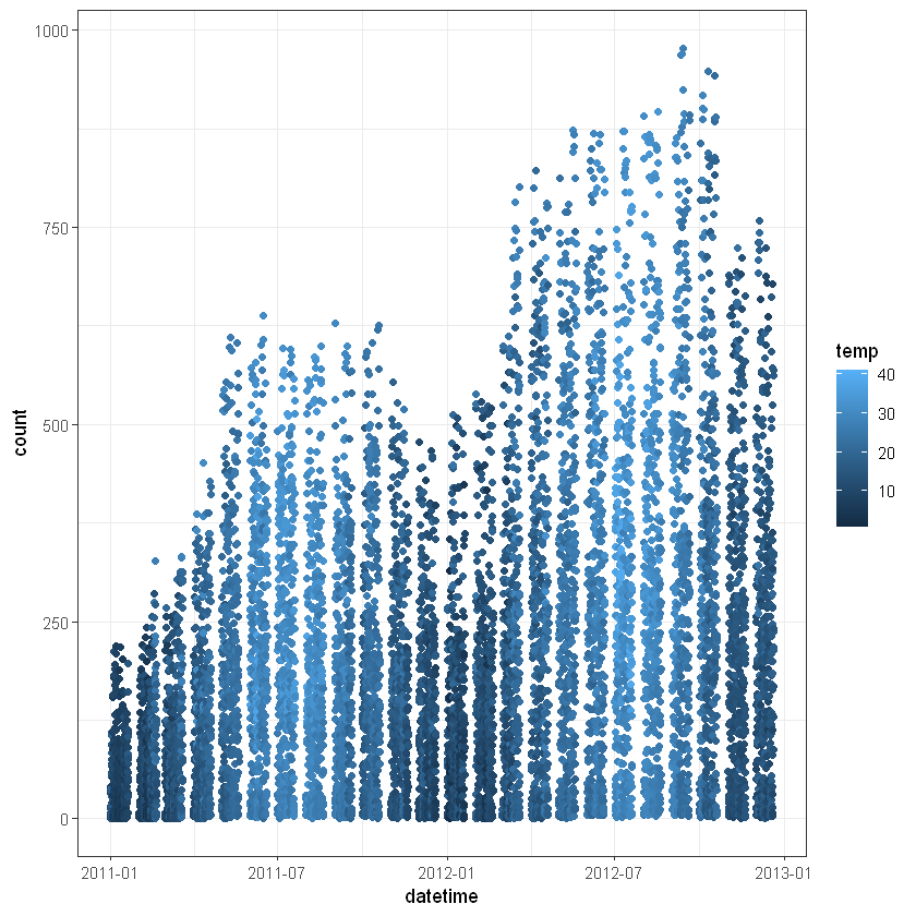
Переглянемо як час оренди байка впливає на кількість замовлень:

ggplot(data, aes(format(datetime, "%H"), count)) + 
        geom_point(aes(color=temp), alpha = 0.5) + 
        theme_bw()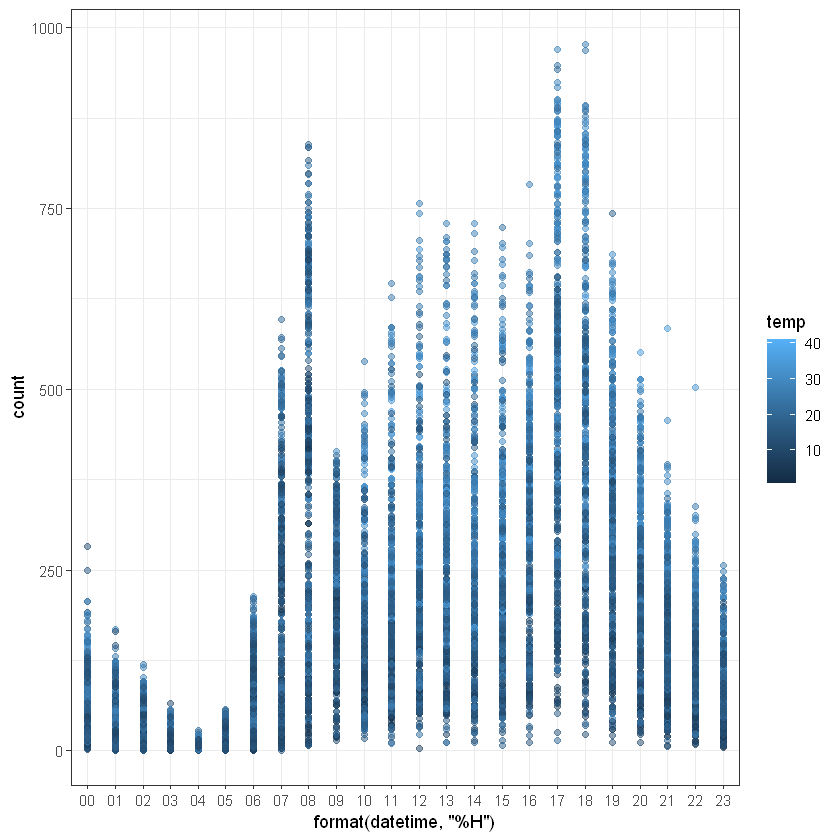

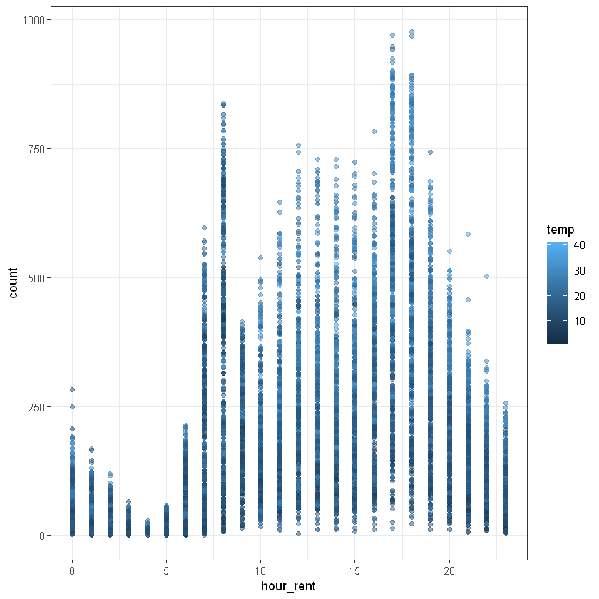
Also, we can add new column to our dataset and use it:

data <- data %>%
    mutate(hour_rent = as.numeric(format(datetime, "%H")))
head(data)

A data.frame: 6 × 11

	datetime	season	holiday	workingday	weather	temp	atemp	humidity	windspeed	count	hour_rent
	<dttm>	<fct>	<fct>	<fct>	<fct>	<dbl>	<dbl>	<int>	<dbl>	<int>	<dbl>
1	2011-01-01 00:00:00	1	0	0	1	9.84	14.395	81	0.0000	16	0
2	2011-01-01 01:00:00	1	0	0	1	9.02	13.635	80	0.0000	40	1
3	2011-01-01 02:00:00	1	0	0	1	9.02	13.635	80	0.0000	32	2
4	2011-01-01 03:00:00	1	0	0	1	9.84	14.395	75	0.0000	13	3
5	2011-01-01 04:00:00	1	0	0	1	9.84	14.395	75	0.0000	1	4
6	2011-01-01 05:00:00	1	0	0	2	9.84	12.880	75	6.0032	1	5

# the same chart as before
ggplot(data, aes(hour_rent, count)) + 
        geom_point(aes(color=temp), alpha = 0.5) + 
        theme_bw()

3.4 Train test split

One more splitting method is based on date. So, we can use first 70% of dataset as train and 30% as test. This method often used for timeseries forecasting. We will use it for linear regression for now.

set.seed(10) 
nrow(data)

train_count = ceiling(0.7 * nrow(data))
train_count

test_count = nrow(data) - train_count
test_count

10886

7621

3265

data <- data %>% arrange(datetime) # sort by datetime

train_data <- data %>% slice_head(n = train_count)
nrow(train_data)
test_data <- data %>% slice_tail(n = test_count)
nrow(test_data)

7621

3265

# lets compare last from train and first from test
tail(train_data)
head(test_data) # ok!

A data.frame: 6 × 11

	datetime	season	holiday	workingday	weather	temp	atemp	humidity	windspeed	count	hour_rent
	<dttm>	<fct>	<fct>	<fct>	<fct>	<dbl>	<dbl>	<int>	<dbl>	<int>	<dbl>
7616	2012-05-16 16:00:00	2	0	1	1	29.52	32.575	45	7.0015	446	16
7617	2012-05-16 17:00:00	2	0	1	1	29.52	33.335	51	12.9980	873	17
7618	2012-05-16 18:00:00	2	0	1	1	29.52	33.335	51	15.0013	846	18
7619	2012-05-16 19:00:00	2	0	1	1	28.70	32.575	54	19.0012	590	19
7620	2012-05-16 20:00:00	2	0	1	1	27.06	31.060	65	16.9979	459	20
7621	2012-05-16 21:00:00	2	0	1	1	26.24	30.305	73	12.9980	393	21

A data.frame: 6 × 11

	datetime	season	holiday	workingday	weather	temp	atemp	humidity	windspeed	count	hour_rent
	<dttm>	<fct>	<fct>	<fct>	<fct>	<dbl>	<dbl>	<int>	<dbl>	<int>	<dbl>
1	2012-05-16 22:00:00	2	0	1	1	26.24	30.305	73	11.0014	286	22
2	2012-05-16 23:00:00	2	0	1	1	25.42	29.545	78	7.0015	133	23
3	2012-05-17 00:00:00	2	0	1	1	24.60	28.790	78	8.9981	79	0
4	2012-05-17 01:00:00	2	0	1	1	24.60	28.030	83	11.0014	28	1
5	2012-05-17 02:00:00	2	0	1	1	24.60	28.790	78	11.0014	16	2
6	2012-05-17 03:00:00	2	0	1	1	24.60	29.545	73	16.9979	3	3

---

3.5 Model building

Побудуємо напройстішу модель залежності середньої температури за день та кількості орендованих байків:

lm_bike <- lm(count ~ atemp, train_data)
summary(lm_bike)

Call:
lm(formula = count ~ atemp, data = train_data)

Residuals:
    Min      1Q  Median      3Q     Max 
-254.42  -93.91  -27.43   65.57  648.09 

Coefficients:
            Estimate Std. Error t value Pr(>|t|)    
(Intercept)  -2.0774     4.4973  -0.462    0.644    
atemp         7.2602     0.1895  38.311   <2e-16 ***
---
Signif. codes:  0 '***' 0.001 '**' 0.01 '*' 0.05 '.' 0.1 ' ' 1

Residual standard error: 138.4 on 7619 degrees of freedom
Multiple R-squared:  0.1615,    Adjusted R-squared:  0.1614 
F-statistic:  1468 on 1 and 7619 DF,  p-value: < 2.2e-16

Спробуємо порахувати кількість орендованих байків для середніх темпертур від 10 до 30 градусів.

Створимо датафрейм з послідовністю елементів 10-30 з кроком 1 та порахуємо за формулою з інформації про модель прогнозовані показники:

Здійснимо прогноз за допомогою функції predict():

#predict_1030$count_model <- predict(lm_bike, newdata = predict_1030)
#predict_1030 %>% head()

# our results are very close, minimal difference is a result of rounding numbers in our formula

# how it looks like at chart
#ggplot(predict_1030, aes(atemp, count_model)) + 
 #       geom_point() + 
    #    theme_bw()

Побудуємо модель для усіх параметрів моделі окрім дати:

lm_bike <- lm(count~.-datetime, train_data)
summary(lm_bike)

Call:
lm(formula = count ~ . - datetime, data = train_data)

Residuals:
    Min      1Q  Median      3Q     Max 
-283.67  -78.72  -25.68   46.27  587.17 

Coefficients:
             Estimate Std. Error t value Pr(>|t|)    
(Intercept)  15.67996    8.85332   1.771   0.0766 .  
season2       9.39674    4.59288   2.046   0.0408 *  
season3     -40.29356    6.46891  -6.229 4.95e-10 ***
season4      21.14562    4.40422   4.801 1.61e-06 ***
holiday1     -8.46508    8.79408  -0.963   0.3358    
workingday1  -4.89327    3.12276  -1.567   0.1172    
weather2      2.76675    3.47283   0.797   0.4257    
weather3    -31.30849    5.61763  -5.573 2.59e-08 ***
weather4     85.56066  122.62585   0.698   0.4854    
temp          1.34075    1.67470   0.801   0.4234    
atemp         6.30809    1.48446   4.249 2.17e-05 ***
humidity     -1.49856    0.08884 -16.868  < 2e-16 ***
windspeed     0.35086    0.19131   1.834   0.0667 .  
hour_rent     6.20760    0.21640  28.685  < 2e-16 ***
---
Signif. codes:  0 '***' 0.001 '**' 0.01 '*' 0.05 '.' 0.1 ' ' 1

Residual standard error: 122.5 on 7607 degrees of freedom
Multiple R-squared:  0.3438,    Adjusted R-squared:  0.3427 
F-statistic: 306.6 on 13 and 7607 DF,  p-value: < 2.2e-16

Перевіримо модель на мультиколінеарність:

suppressMessages(library(car))
vif(lm_bike)

A matrix: 9 × 3 of type dbl

	GVIF	Df	GVIF^(1/(2*Df))
season	2.941744	3	1.197018
holiday	1.076162	1	1.037382
workingday	1.072163	1	1.035453
weather	1.291207	3	1.043516
temp	83.073739	1	9.114480
atemp	78.281362	1	8.847676
humidity	1.594124	1	1.262586
windspeed	1.331723	1	1.154003
hour_rent	1.135437	1	1.065569

Виключимо корельовані показники з моделі за принципом - залишити той, що має вищу кореляцію із залежним фактором. У нашому випадку це temp:

lm_bike <- lm(count~.-datetime-atemp, train_data)
summary(lm_bike)

Call:
lm(formula = count ~ . - datetime - atemp, data = train_data)

Residuals:
    Min      1Q  Median      3Q     Max 
-297.02  -79.11  -25.60   46.35  585.12 

Coefficients:
             Estimate Std. Error t value Pr(>|t|)    
(Intercept)  26.97221    8.45456   3.190  0.00143 ** 
season2       9.25257    4.59790   2.012  0.04422 *  
season3     -45.22396    6.37114  -7.098 1.38e-12 ***
season4      22.00064    4.40455   4.995 6.02e-07 ***
holiday1    -11.34365    8.77778  -1.292  0.19629    
workingday1  -4.86349    3.12625  -1.556  0.11982    
weather2      3.02977    3.47616   0.872  0.38346    
weather3    -32.19037    5.62008  -5.728 1.06e-08 ***
weather4     88.33390  122.76150   0.720  0.47182    
temp          8.34447    0.29736  28.062  < 2e-16 ***
humidity     -1.47674    0.08879 -16.632  < 2e-16 ***
windspeed     0.06683    0.17945   0.372  0.70959    
hour_rent     6.20731    0.21665  28.652  < 2e-16 ***
---
Signif. codes:  0 '***' 0.001 '**' 0.01 '*' 0.05 '.' 0.1 ' ' 1

Residual standard error: 122.7 on 7608 degrees of freedom
Multiple R-squared:  0.3422,    Adjusted R-squared:  0.3412 
F-statistic: 329.9 on 12 and 7608 DF,  p-value: < 2.2e-16

Далі побудуємо модель на основі алгоритму stepwise та порівняємо з поточними характеристиками моделі.

Створимо моделі для проходів у два боки:

start_mod <- lm(count ~ 1, data = train_data)
end_mod <- lm(count ~ . - datetime - temp, data = train_data)

Запустимо алгоритм функцією step():

lm_bike_stepwise <- step(start_mod,
                     scope = list(lower = start_mod, upper = end_mod),
                     direction = "both", trace = 1, steps = 1000)

Start:  AIC=76488.12
count ~ 1

             Df Sum of Sq       RSS   AIC
+ atemp       1  28114587 145942663 75148
+ hour_rent   1  27600736 146456514 75174
+ humidity    1  15503642 158553609 75779
+ season      3   9131936 164925314 76083
+ weather     3   3537078 170520172 76338
+ windspeed   1   2112392 171944858 76397
<none>                    174057250 76488
+ holiday     1     12170 174045081 76490
+ workingday  1      3511 174053739 76490

Step:  AIC=75147.53
count ~ atemp

             Df Sum of Sq       RSS   AIC
+ hour_rent   1  20603748 125338915 73990
+ humidity    1  15576942 130365721 74289
+ season      3   5178271 140764392 74878
+ weather     3   2989985 142952678 74996
+ windspeed   1   2889374 143053289 74997
<none>                    145942663 75148
+ workingday  1     34765 145907898 75148
+ holiday     1        44 145942619 75150
- atemp       1  28114587 174057250 76488

Step:  AIC=73989.67
count ~ atemp + hour_rent

             Df Sum of Sq       RSS   AIC
+ humidity    1   8093815 117245100 73483
+ season      3   2905720 122433195 73817
+ weather     3   2861080 122477834 73820
+ windspeed   1   1038961 124299954 73928
<none>                    125338915 73990
+ workingday  1     29661 125309254 73990
+ holiday     1       313 125338602 73992
- hour_rent   1  20603748 145942663 75148
- atemp       1  21117599 146456514 75174

Step:  AIC=73482.93
count ~ atemp + hour_rent + humidity

             Df Sum of Sq       RSS   AIC
+ season      3   2375796 114869304 73333
+ weather     3    534048 116711052 73454
+ workingday  1     32372 117212728 73483
<none>                    117245100 73483
+ windspeed   1     22790 117222310 73483
+ holiday     1      6750 117238350 73484
- humidity    1   8093815 125338915 73990
- hour_rent   1  13120621 130365721 74289
- atemp       1  22173444 139418544 74801

Step:  AIC=73332.92
count ~ atemp + hour_rent + humidity + season

             Df Sum of Sq       RSS   AIC
+ weather     3    525600 114343704 73304
+ workingday  1     42319 114826985 73332
+ windspeed   1     31234 114838071 73333
<none>                    114869304 73333
+ holiday     1      2238 114867066 73335
- season      3   2375796 117245100 73483
- humidity    1   7563890 122433195 73817
- atemp       1  12150238 127019542 74097
- hour_rent   1  12266423 127135727 74104

Step:  AIC=73303.97
count ~ atemp + hour_rent + humidity + season + weather

             Df Sum of Sq       RSS   AIC
+ windspeed   1     77129 114266576 73301
+ workingday  1     30192 114313512 73304
<none>                    114343704 73304
+ holiday     1      3786 114339918 73306
- weather     3    525600 114869304 73333
- season      3   2367348 116711052 73454
- humidity    1   5224113 119567817 73642
- atemp       1  12055477 126399182 74066
- hour_rent   1  12568342 126912046 74097

Step:  AIC=73300.82
count ~ atemp + hour_rent + humidity + season + weather + windspeed

             Df Sum of Sq       RSS   AIC
<none>                    114266576 73301
+ workingday  1     28599 114237977 73301
+ holiday     1      4334 114262242 73303
- windspeed   1     77129 114343704 73304
- weather     3    571495 114838071 73333
- season      3   2382626 116649202 73452
- humidity    1   4315759 118582335 73581
- atemp       1  12116310 126382885 74067
- hour_rent   1  12411506 126678081 74085

# check the summary
summary(lm_bike_stepwise)

Call:
lm(formula = count ~ atemp + hour_rent + humidity + season + 
    weather + windspeed, data = train_data)

Residuals:
    Min      1Q  Median      3Q     Max 
-285.56  -78.70  -25.63   47.20  586.14 

Coefficients:
             Estimate Std. Error t value Pr(>|t|)    
(Intercept)  10.56655    8.35898   1.264   0.2062    
atemp         7.46224    0.26269  28.407  < 2e-16 ***
hour_rent     6.21766    0.21626  28.750  < 2e-16 ***
humidity     -1.50051    0.08851 -16.954  < 2e-16 ***
season2       9.95637    4.55753   2.185   0.0289 *  
season3     -38.55100    6.14342  -6.275 3.68e-10 ***
season4      21.22676    4.40003   4.824 1.43e-06 ***
weather2      2.68041    3.47136   0.772   0.4400    
weather3    -31.47986    5.60817  -5.613 2.06e-08 ***
weather4     83.31112  122.62122   0.679   0.4969    
windspeed     0.40641    0.17932   2.266   0.0235 *  
---
Signif. codes:  0 '***' 0.001 '**' 0.01 '*' 0.05 '.' 0.1 ' ' 1

Residual standard error: 122.5 on 7610 degrees of freedom
Multiple R-squared:  0.3435,    Adjusted R-squared:  0.3426 
F-statistic: 398.2 on 10 and 7610 DF,  p-value: < 2.2e-16

\(R^2\) increses!

Об’єднаємо для наочності коефіцієнти у один датафрейм:

lm_coefs_def <- data.frame(lm_name = names(lm_bike$coefficients),
                           name = lm_bike$coefficients, 
                           row.names = c() # cleaning rownames
                          )
lm_coefs_def

A data.frame: 13 × 2

lm_name	name
<chr>	<dbl>
(Intercept)	26.97221255
season2	9.25256711
season3	-45.22395805
season4	22.00064078
holiday1	-11.34364536
workingday1	-4.86348665
weather2	3.02977126
weather3	-32.19036573
weather4	88.33390060
temp	8.34447012
humidity	-1.47674448
windspeed	0.06683245
hour_rent	6.20730753

lm_coefs_sw <- data.frame(lm_name = names(lm_bike_stepwise$coefficients), name = lm_bike_stepwise$coefficients, row.names = c())
lm_coefs_sw

A data.frame: 11 × 2

lm_name	name
<chr>	<dbl>
(Intercept)	10.5665521
atemp	7.4622378
hour_rent	6.2176579
humidity	-1.5005074
season2	9.9563690
season3	-38.5510028
season4	21.2267554
weather2	2.6804117
weather3	-31.4798561
weather4	83.3111193
windspeed	0.4064147

# lets combine coefficients from both models
lm_coefs <- merge(lm_coefs_def, lm_coefs_sw, by = "lm_name", X.all = T, X.all = T)
colnames(lm_coefs) <- c("variable", "lm", "lm_sw")
lm_coefs

A data.frame: 10 × 3

variable	lm	lm_sw
<chr>	<dbl>	<dbl>
(Intercept)	26.97221255	10.5665521
hour_rent	6.20730753	6.2176579
humidity	-1.47674448	-1.5005074
season2	9.25256711	9.9563690
season3	-45.22395805	-38.5510028
season4	22.00064078	21.2267554
weather2	3.02977126	2.6804117
weather3	-32.19036573	-31.4798561
weather4	88.33390060	83.3111193
windspeed	0.06683245	0.4064147

Як бачимо моделі мають незначні відмінності.

---

3.6 Model errors analysis

Запишемо у train набір даних модельовані значення count та похибки:

train_data$predicted <- lm_bike$fitted.values
train_data$residuals <- lm_bike$residuals
head(train_data)

A data.frame: 6 × 13

	datetime	season	holiday	workingday	weather	temp	atemp	humidity	windspeed	count	hour_rent	predicted	residuals
	<dttm>	<fct>	<fct>	<fct>	<fct>	<dbl>	<dbl>	<int>	<dbl>	<int>	<dbl>	<dbl>	<dbl>
1	2011-01-01 00:00:00	1	0	0	1	9.84	14.395	81	0.0000	16	0	-10.534505	26.534505
2	2011-01-01 01:00:00	1	0	0	1	9.02	13.635	80	0.0000	40	1	-9.692918	49.692918
3	2011-01-01 02:00:00	1	0	0	1	9.02	13.635	80	0.0000	32	2	-3.485611	35.485611
4	2011-01-01 03:00:00	1	0	0	1	9.84	14.395	75	0.0000	13	3	16.947885	-3.947885
5	2011-01-01 04:00:00	1	0	0	1	9.84	14.395	75	0.0000	1	4	23.155192	-22.155192
6	2011-01-01 05:00:00	1	0	0	2	9.84	12.880	75	6.0032	1	5	32.793480	-31.793480

Візуалізуємо відхилення моделі:

plot_data <- train_data[1:100,]

ggplot(plot_data, aes(x = c(1:nrow(plot_data)), y = as.numeric(count))) +
  geom_segment(aes(xend = c(1:nrow(plot_data)), yend = predicted), alpha = .2) +
  geom_point(aes(color = residuals), size = 2) +
  scale_color_gradient2(low = "blue", mid = "white", high = "red") +
  guides(color = FALSE) +
  geom_point(aes(y = predicted), shape = 1, size = 2) +
  geom_hline(yintercept=0.5, linetype="dashed", color = "red") +
  theme_bw()

Warning message:
"`guides(<scale> = FALSE)` is deprecated. Please use `guides(<scale> = "none")` instead."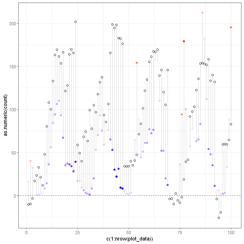

Lets check the same for test data

First we need to predict values:

test_data$predicted <- predict(lm_bike, newdata = test_data)
head(test_data)

A data.frame: 6 × 12

	datetime	season	holiday	workingday	weather	temp	atemp	humidity	windspeed	count	hour_rent	predicted
	<dttm>	<fct>	<fct>	<fct>	<fct>	<dbl>	<dbl>	<int>	<dbl>	<int>	<dbl>	<dbl>
1	2012-05-16 22:00:00	2	0	1	1	26.24	30.305	73	11.0014	286	22	279.8139
2	2012-05-16 23:00:00	2	0	1	1	25.42	29.545	78	7.0015	133	23	271.5277
3	2012-05-17 00:00:00	2	0	1	1	24.60	28.790	78	8.9981	79	0	122.0506
4	2012-05-17 01:00:00	2	0	1	1	24.60	28.030	83	11.0014	28	1	121.0080
5	2012-05-17 02:00:00	2	0	1	1	24.60	28.790	78	11.0014	16	2	134.5991
6	2012-05-17 03:00:00	2	0	1	1	24.60	29.545	73	16.9979	3	3	148.5908

# resulduals calculation
test_data$residuals <- test_data$count - test_data$predicted
head(test_data)

A data.frame: 6 × 13

	datetime	season	holiday	workingday	weather	temp	atemp	humidity	windspeed	count	hour_rent	predicted	residuals
	<dttm>	<fct>	<fct>	<fct>	<fct>	<dbl>	<dbl>	<int>	<dbl>	<int>	<dbl>	<dbl>	<dbl>
1	2012-05-16 22:00:00	2	0	1	1	26.24	30.305	73	11.0014	286	22	279.8139	6.186142
2	2012-05-16 23:00:00	2	0	1	1	25.42	29.545	78	7.0015	133	23	271.5277	-138.527654
3	2012-05-17 00:00:00	2	0	1	1	24.60	28.790	78	8.9981	79	0	122.0506	-43.050553
4	2012-05-17 01:00:00	2	0	1	1	24.60	28.030	83	11.0014	28	1	121.0080	-93.008024
5	2012-05-17 02:00:00	2	0	1	1	24.60	28.790	78	11.0014	16	2	134.5991	-118.599054
6	2012-05-17 03:00:00	2	0	1	1	24.60	29.545	73	16.9979	3	3	148.5908	-145.590844

plot_data <- test_data[1:100,]

ggplot(plot_data, aes(x = c(1:nrow(plot_data)), y = as.numeric(count))) +
  geom_segment(aes(xend = c(1:nrow(plot_data)), yend = predicted), alpha = .2) +
  geom_point(aes(color = residuals), size = 2) +
  scale_color_gradient2(low = "blue", mid = "white", high = "red") +
  guides(color = FALSE) +
  geom_point(aes(y = predicted), shape = 1, size = 2) +
  geom_hline(yintercept=0.5, linetype="dashed", color = "red") +
  theme_bw()

Warning message:
"`guides(<scale> = FALSE)` is deprecated. Please use `guides(<scale> = "none")` instead."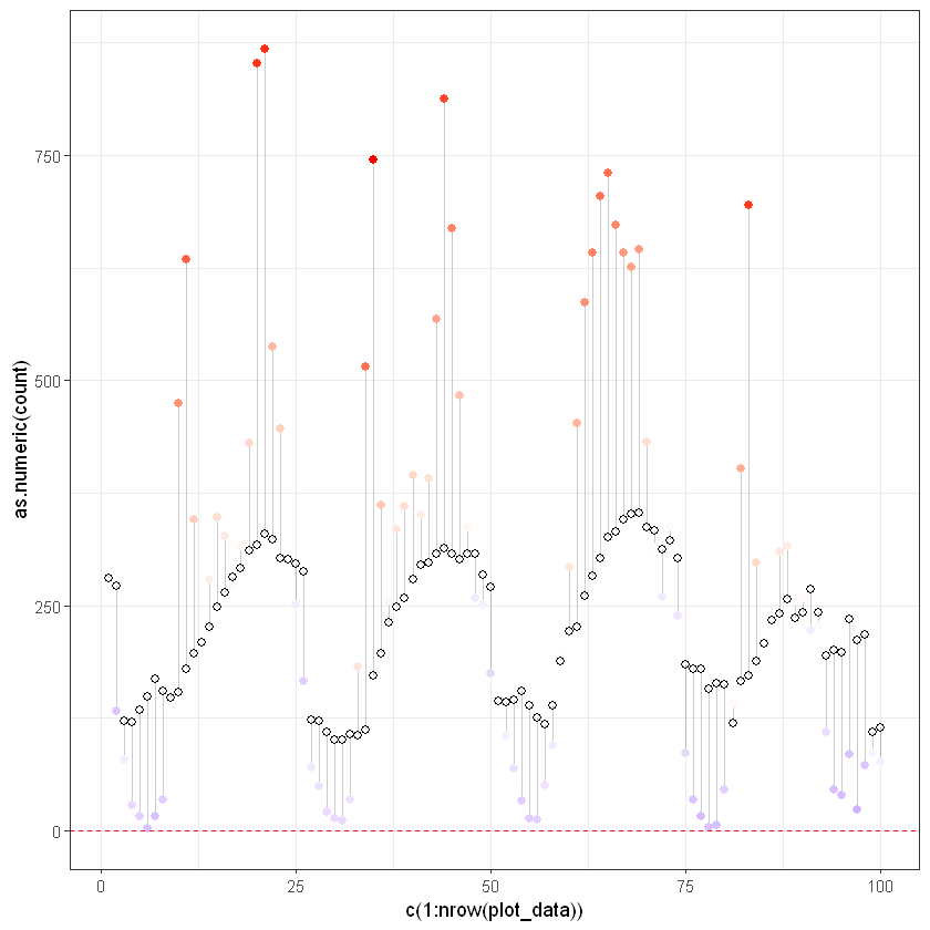

library(modelr)
resids <- data.frame(
  R2 = c(rsquare(lm_bike, data = train_data), rsquare(lm_bike, data = test_data)),
  MSE = c(mse(lm_bike, data = train_data),mse(lm_bike, data = test_data)),
  RMSE = c(rmse(lm_bike, data = train_data), rmse(lm_bike, data = test_data))#,
  #MAE = c(mae(lm_bike, data = train_data), mae(lm_bike, data = test_data)), # if needed 
  #MAPE = c(mape(lm_bike, data = train_data), mape(lm_bike, data = test_data)) # if needed
)
          
rownames(resids) <- c("train", "test") # give names for rows

resids

A data.frame: 2 × 3

	R2	MSE	RMSE
	<dbl>	<dbl>	<dbl>
train	0.3422443	15022.59	122.5667
test	0.2854741	40401.94	201.0023

Conclusion: Test set has less RSquared and Bigger Errors variation. Train dataset is closer, because it built on training data and model include information about data.

---