8  Нейронні мережі. Deep Learning. Класифікація. Кредитний скоринг

Курс: “Математичне моделювання в R”

---

Sys.setlocale("LC_CTYPE", "ukrainian") 
options(warn = -1)

'Ukrainian_Ukraine.1251'

8.1 Набір даних

Джерело: https://www.kaggle.com/barelydedicated/bank-customer-churn-modeling.

Завантажимо файли з даними:

customers <- read.csv("data/customers.csv")
products <- read.csv("data/products.csv")
cards <- read.csv("data/cards.csv")

Цей датасет містить такі стовпці:

• RowNumber - номер рядка.
• CustomerId - ідентифікатор клієнта.
• Surname - прізвище клієнта.
• CreditScore - кредитний рейтинг клієнта.
• Geography - регіон.
• Gender - стать.
• Age - вік.
• Tenure - час обслуговування цього клієнта в банку.
• IsActiveMember - активний клієнт, виконує операції.
• EstimatedSalary - заробітна плата.
• Exited - залишив/не залишив банк.

Інформація про клієнтів:

str(customers)

'data.frame':   10000 obs. of  11 variables:
 $ RowNumber      : int  1 2 3 4 5 6 7 8 9 10 ...
 $ CustomerId     : int  15634602 15647311 15619304 15701354 15737888 15574012 15592531 15656148 15792365 15592389 ...
 $ Surname        : chr  "Hargrave" "Hill" "Onio" "Boni" ...
 $ CreditScore    : int  619 608 502 699 850 645 822 376 501 684 ...
 $ Geography      : chr  "France" "Spain" "France" "France" ...
 $ Gender         : chr  "Female" "Female" "Female" "Female" ...
 $ Age            : int  42 41 42 39 43 44 50 29 44 27 ...
 $ Tenure         : int  2 1 8 1 2 8 7 4 4 2 ...
 $ IsActiveMember : int  1 1 0 0 1 0 1 0 1 1 ...
 $ EstimatedSalary: num  101349 112543 113932 93827 79084 ...
 $ Exited         : int  1 0 1 0 0 1 0 1 0 0 ...

head(customers)

A data.frame: 6 × 11

	RowNumber	CustomerId	Surname	CreditScore	Geography	Gender	Age	Tenure	IsActiveMember	EstimatedSalary	Exited
	<int>	<int>	<chr>	<int>	<chr>	<chr>	<int>	<int>	<int>	<dbl>	<int>
1	1	15634602	Hargrave	619	France	Female	42	2	1	101348.88	1
2	2	15647311	Hill	608	Spain	Female	41	1	1	112542.58	0
3	3	15619304	Onio	502	France	Female	42	8	0	113931.57	1
4	4	15701354	Boni	699	France	Female	39	1	0	93826.63	0
5	5	15737888	Mitchell	850	Spain	Female	43	2	1	79084.10	0
6	6	15574012	Chu	645	Spain	Male	44	8	0	149756.71	1

8.2 Оглядовий аналіз даних

8.2.1 Таблиця customers

Оглянемо дані колекції customers візуально та за допомогою крос-таблиць:

library(gmodels)
library(ggplot2)

Кредитний рейтинг (CreditScore):

ggplot(customers, aes(x=CreditScore, fill=factor(Exited))) + 
  geom_histogram(binwidth = 10, alpha=0.7) + theme_bw()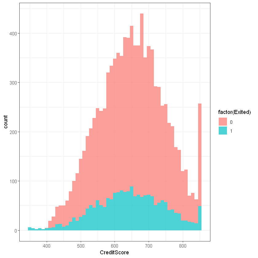 

Регіон/країна (Geography):

ggplot(customers, aes(x=Geography, fill=factor(Exited))) + 
  geom_bar(position = "stack") + theme_bw()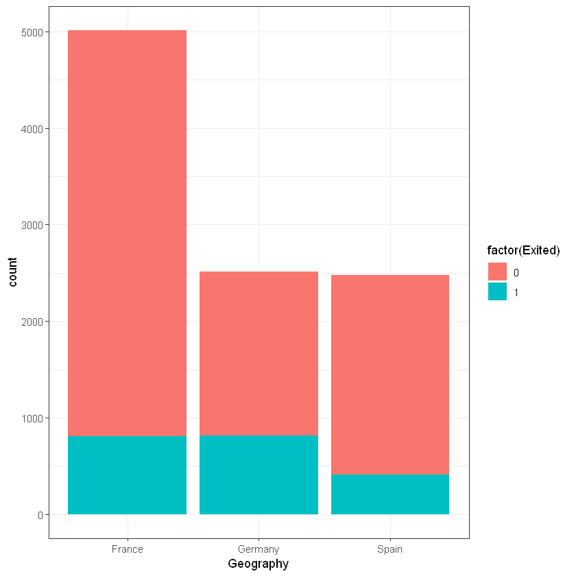

CrossTable(customers$Geography, customers$Exited)

 
   Cell Contents
|-------------------------|
|                       N |
| Chi-square contribution |
|           N / Row Total |
|           N / Col Total |
|         N / Table Total |
|-------------------------|

 
Total Observations in Table:  10000 

 
                    | customers$Exited 
customers$Geography |         0 |         1 | Row Total | 
--------------------|-----------|-----------|-----------|
             France |      4204 |       810 |      5014 | 
                    |    11.188 |    43.736 |           | 
                    |     0.838 |     0.162 |     0.501 | 
                    |     0.528 |     0.398 |           | 
                    |     0.420 |     0.081 |           | 
--------------------|-----------|-----------|-----------|
            Germany |      1695 |       814 |      2509 | 
                    |    45.927 |   179.537 |           | 
                    |     0.676 |     0.324 |     0.251 | 
                    |     0.213 |     0.400 |           | 
                    |     0.170 |     0.081 |           | 
--------------------|-----------|-----------|-----------|
              Spain |      2064 |       413 |      2477 | 
                    |     4.251 |    16.617 |           | 
                    |     0.833 |     0.167 |     0.248 | 
                    |     0.259 |     0.203 |           | 
                    |     0.206 |     0.041 |           | 
--------------------|-----------|-----------|-----------|
       Column Total |      7963 |      2037 |     10000 | 
                    |     0.796 |     0.204 |           | 
--------------------|-----------|-----------|-----------|

 

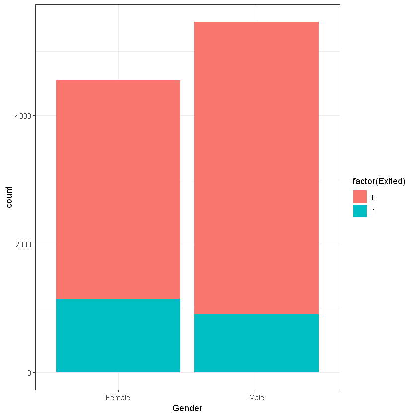
Стать (Gender):

ggplot(customers, aes(x=Gender, fill=factor(Exited))) + 
  geom_bar(position = "stack") + theme_bw()

CrossTable(customers$Gender, customers$Exited)

 
   Cell Contents
|-------------------------|
|                       N |
| Chi-square contribution |
|           N / Row Total |
|           N / Col Total |
|         N / Table Total |
|-------------------------|

 
Total Observations in Table:  10000 

 
                 | customers$Exited 
customers$Gender |         0 |         1 | Row Total | 
-----------------|-----------|-----------|-----------|
          Female |      3404 |      1139 |      4543 | 
                 |    12.611 |    49.298 |           | 
                 |     0.749 |     0.251 |     0.454 | 
                 |     0.427 |     0.559 |           | 
                 |     0.340 |     0.114 |           | 
-----------------|-----------|-----------|-----------|
            Male |      4559 |       898 |      5457 | 
                 |    10.499 |    41.041 |           | 
                 |     0.835 |     0.165 |     0.546 | 
                 |     0.573 |     0.441 |           | 
                 |     0.456 |     0.090 |           | 
-----------------|-----------|-----------|-----------|
    Column Total |      7963 |      2037 |     10000 | 
                 |     0.796 |     0.204 |           | 
-----------------|-----------|-----------|-----------|

 

Вік (Age):

ggplot(customers, aes(x=Age, fill=factor(Exited))) + 
  geom_histogram(binwidth = 1, alpha=0.7) + theme_bw()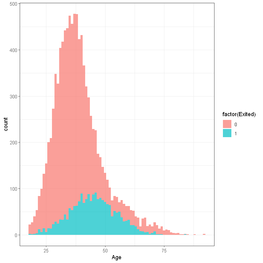 

Час обслуговування клієнта (Tenure):

ggplot(customers, aes(x=Tenure, fill=factor(Exited))) + 
  geom_histogram(binwidth = 1, alpha=0.7) + theme_bw()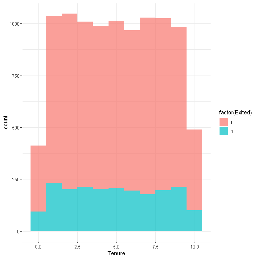 

Активність (IsActiveMember):

CrossTable(customers$IsActiveMember, customers$Exited)

 
   Cell Contents
|-------------------------|
|                       N |
| Chi-square contribution |
|           N / Row Total |
|           N / Col Total |
|         N / Table Total |
|-------------------------|

 
Total Observations in Table:  10000 

 
                         | customers$Exited 
customers$IsActiveMember |         0 |         1 | Row Total | 
-------------------------|-----------|-----------|-----------|
                       0 |      3547 |      1302 |      4849 | 
                         |    25.577 |    99.984 |           | 
                         |     0.731 |     0.269 |     0.485 | 
                         |     0.445 |     0.639 |           | 
                         |     0.355 |     0.130 |           | 
-------------------------|-----------|-----------|-----------|
                       1 |      4416 |       735 |      5151 | 
                         |    24.077 |    94.122 |           | 
                         |     0.857 |     0.143 |     0.515 | 
                         |     0.555 |     0.361 |           | 
                         |     0.442 |     0.073 |           | 
-------------------------|-----------|-----------|-----------|
            Column Total |      7963 |      2037 |     10000 | 
                         |     0.796 |     0.204 |           | 
-------------------------|-----------|-----------|-----------|

 

Заробітна плата (EstimatedSalary):

ggplot(customers, aes(x=EstimatedSalary, fill=factor(Exited))) + 
  geom_histogram(binwidth = 1000, alpha=0.7) + theme_bw()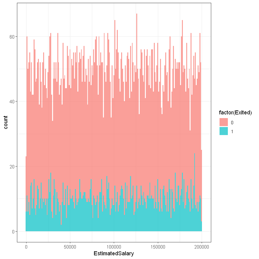 

Exited:

CrossTable(customers$Exited)

 
   Cell Contents
|-------------------------|
|                       N |
|         N / Table Total |
|-------------------------|

 
Total Observations in Table:  10000 

 
          |         0 |         1 | 
          |-----------|-----------|
          |      7963 |      2037 | 
          |     0.796 |     0.204 | 
          |-----------|-----------|



 

---

8.2.2 Таблиця cards

Інформація про карти клієнта:

str(cards)

'data.frame':   13545 obs. of  4 variables:
 $ CustomerId  : int  15634602 15647311 15647311 15619304 15619304 15701354 15701354 15737888 15737888 15574012 ...
 $ CardNo      : int  684618 357092 802678 888594 987103 507476 928960 370210 935036 581042 ...
 $ IsCreditCard: int  1 0 0 1 0 0 0 1 0 1 ...
 $ Balance     : num  5 41922 41913 79846 79859 ...

head(cards)

A data.frame: 6 × 4

	CustomerId	CardNo	IsCreditCard	Balance
	<int>	<int>	<int>	<dbl>
1	15634602	684618	1	5.00
2	15647311	357092	0	41921.93
3	15647311	802678	0	41912.93
4	15619304	888594	1	79846.40
5	15619304	987103	0	79859.40
6	15701354	507476	0	28.00

summary(cards)

   CustomerId           CardNo        IsCreditCard       Balance      
 Min.   :15565701   Min.   :100231   Min.   :0.0000   Min.   :     0  
 1st Qu.:15628272   1st Qu.:323587   1st Qu.:0.0000   1st Qu.:    24  
 Median :15691011   Median :545073   Median :0.0000   Median : 52991  
 Mean   :15690848   Mean   :548414   Mean   :0.4688   Mean   : 51096  
 3rd Qu.:15752816   3rd Qu.:774943   3rd Qu.:1.0000   3rd Qu.: 77276  
 Max.   :15815690   Max.   :999985   Max.   :1.0000   Max.   :221549  

---

8.2.3 Таблиця products

Інформація про продукти клієнта:

str(products)

'data.frame':   13862 obs. of  2 variables:
 $ CustomerId : int  15634602 15647311 15619304 15619304 15619304 15701354 15701354 15737888 15574012 15574012 ...
 $ ProductName: chr  "PROD_1" "PROD_1" "PROD_1" "PROD_2" ...

head(products)

A data.frame: 6 × 2

	CustomerId	ProductName
	<int>	<chr>
1	15634602	PROD_1
2	15647311	PROD_1
3	15619304	PROD_1
4	15619304	PROD_2
5	15619304	PROD_3
6	15701354	PROD_1

---

8.3 Feature engeniering

Сформуємо додаткові змінні на основі наявних даних:

• Balance - сума по усіх картах клієнат.
• NumOfProducts - кількість продуктів банку, які використовує клієнт.
• HasCreditCard - dummy-змінна, наявність кредитної карти у клієнта.

8.3.1 Показник NumOfProducts

Варто звернути увагу, що генерувати нові фічі можна із використанням можлиовстей агрегації та фільтрування даних (наприклад, методи пакету dplyr) або за допомогою простих алгоритмічних структур (цикли, розгалуження).

Для R використання циклів для подібних задач є не досить хорошим рішенням, адже код виглядає складно і виконується повільно. Проте ми напишемо для требування і пояснення приклади з використанням обох підходів.

Імперативний підхід до програмування:

# Створюємо пусту змінну
customers$NumOfProducts <- c(0)

for(i in 1:nrow(customers))
{
  id <- customers$CustomerId[i]
  prods <- subset(products, CustomerId == id)
  customers$NumOfProducts[i] <- nrow(prods)
}

head(customers, 4)

A data.frame: 4 × 12

	RowNumber	CustomerId	Surname	CreditScore	Geography	Gender	Age	Tenure	IsActiveMember	EstimatedSalary	Exited	NumOfProducts
	<int>	<int>	<chr>	<int>	<chr>	<chr>	<int>	<int>	<int>	<dbl>	<int>	<dbl>
1	1	15634602	Hargrave	619	France	Female	42	2	1	101348.88	1	1
2	2	15647311	Hill	608	Spain	Female	41	1	1	112542.58	0	1
3	3	15619304	Onio	502	France	Female	42	8	0	113931.57	1	3
4	4	15701354	Boni	699	France	Female	39	1	0	93826.63	0	2

Декларативний приклад коду:

suppressMessages(library(dplyr))

customers_tmp <- customers |>
    left_join(products |> 
              group_by(CustomerId) |> 
              mutate(NumOfProducts = n()) |>
              select(CustomerId, NumOfProducts) |> distinct(), by = "CustomerId")

head(customers_tmp, 4)

# P.S. Це набагато швидше

A data.frame: 4 × 13

	RowNumber	CustomerId	Surname	CreditScore	Geography	Gender	Age	Tenure	IsActiveMember	EstimatedSalary	Exited	NumOfProducts.x	NumOfProducts.y
	<int>	<int>	<chr>	<int>	<chr>	<chr>	<int>	<int>	<int>	<dbl>	<int>	<dbl>	<int>
1	1	15634602	Hargrave	619	France	Female	42	2	1	101348.88	1	1	1
2	2	15647311	Hill	608	Spain	Female	41	1	1	112542.58	0	1	1
3	3	15619304	Onio	502	France	Female	42	8	0	113931.57	1	3	3
4	4	15701354	Boni	699	France	Female	39	1	0	93826.63	0	2	2

---

8.3.2 Показник HasCreditCard

customers <- customers |>
    left_join(cards |> 
              group_by(CustomerId) |> 
              summarise(HasCreditCard = ifelse(sum(IsCreditCard) == 0, 0, 1)) |>
              select(CustomerId, HasCreditCard) |> distinct(), by = "CustomerId")

head(customers, 4)

A data.frame: 4 × 13

	RowNumber	CustomerId	Surname	CreditScore	Geography	Gender	Age	Tenure	IsActiveMember	EstimatedSalary	Exited	NumOfProducts	HasCreditCard
	<int>	<int>	<chr>	<int>	<chr>	<chr>	<int>	<int>	<int>	<dbl>	<int>	<dbl>	<dbl>
1	1	15634602	Hargrave	619	France	Female	42	2	1	101348.88	1	1	1
2	2	15647311	Hill	608	Spain	Female	41	1	1	112542.58	0	1	0
3	3	15619304	Onio	502	France	Female	42	8	0	113931.57	1	3	1
4	4	15701354	Boni	699	France	Female	39	1	0	93826.63	0	2	0

---

8.3.3 Показник Balance

customers <- customers |>
    left_join(cards |> 
              group_by(CustomerId) |> 
              mutate(Balance = round(sum(Balance))) |>
              select(CustomerId, Balance) |> distinct(), by = "CustomerId")

head(customers, 4)

A data.frame: 4 × 14

	RowNumber	CustomerId	Surname	CreditScore	Geography	Gender	Age	Tenure	IsActiveMember	EstimatedSalary	Exited	NumOfProducts	HasCreditCard	Balance
	<int>	<int>	<chr>	<int>	<chr>	<chr>	<int>	<int>	<int>	<dbl>	<int>	<dbl>	<dbl>	<dbl>
1	1	15634602	Hargrave	619	France	Female	42	2	1	101348.88	1	1	1	5
2	2	15647311	Hill	608	Spain	Female	41	1	1	112542.58	0	1	0	83835
3	3	15619304	Onio	502	France	Female	42	8	0	113931.57	1	3	1	159706
4	4	15701354	Boni	699	France	Female	39	1	0	93826.63	0	2	0	47

Звичано код можна поєднати в 1 запит.

8.3.4 Нормалізація даних

Видалимо зайві покзники, що заважатимуть будувати моделі:

customers <- customers |>
    dplyr::select(-c(RowNumber, CustomerId, Surname))

Варто звернути увагу, що інженереія нових фіч завершена не до кінця і у нас ще присутні параметри, що мають нечислові значення Geography + Gender. Спробуйте замінити їх, наприклад, на dummy-змінні або використати бінінг.

Для скорочення часу на вивчення матеріали ми скористаємося звичайним приведенням даних до числового типу:

customers$Geography <- as.numeric(as.factor(customers$Geography))
customers$Gender <- as.numeric(as.factor(customers$Gender))

str(customers)

'data.frame':   10000 obs. of  11 variables:
 $ CreditScore    : int  619 608 502 699 850 645 822 376 501 684 ...
 $ Geography      : num  1 3 1 1 3 3 1 2 1 1 ...
 $ Gender         : num  1 1 1 1 1 2 2 1 2 2 ...
 $ Age            : int  42 41 42 39 43 44 50 29 44 27 ...
 $ Tenure         : int  2 1 8 1 2 8 7 4 4 2 ...
 $ IsActiveMember : int  1 1 0 0 1 0 1 0 1 1 ...
 $ EstimatedSalary: num  101349 112543 113932 93827 79084 ...
 $ Exited         : int  1 0 1 0 0 1 0 1 0 0 ...
 $ NumOfProducts  : num  1 1 3 2 1 2 2 4 2 1 ...
 $ HasCreditCard  : num  1 0 1 0 1 1 1 1 0 1 ...
 $ Balance        : num  5 83835 159706 47 125571 ...

Використовуючи функцію scale() нормалізуємо дані:

scaled <- scale(customers[-8], center = TRUE)
scaled <- cbind(scaled, customers[8])
head(scaled,)

A data.frame: 6 × 11

	CreditScore	Geography	Gender	Age	Tenure	IsActiveMember	EstimatedSalary	NumOfProducts	HasCreditCard	Balance	Exited
	<dbl>	<dbl>	<dbl>	<dbl>	<dbl>	<dbl>	<dbl>	<dbl>	<dbl>	<dbl>	<int>
1	-0.32620511	-0.9018411	-1.0959327	0.293502747	-1.041708	0.970194	0.0218854	-0.5420116	0.6521559	-1.2240103	1
2	-0.44001395	1.5149916	-1.0959327	0.198153924	-1.387468	0.970194	0.2165229	-0.5420116	-1.5332062	0.1179507	0
3	-1.53671734	-0.9018411	-1.0959327	0.293502747	1.032856	-1.030619	0.2406749	2.2648841	0.6521559	1.3325030	1
4	0.50149556	-0.9018411	-1.0959327	0.007456278	-1.387468	-1.030619	-0.1089125	0.8614363	-1.5332062	-1.2233380	0
5	2.06378057	1.5149916	-1.0959327	0.388851570	-1.041708	0.970194	-0.3652575	-0.5420116	0.6521559	0.7860657	0
6	-0.05720239	1.5149916	0.9123735	0.484200392	1.032856	-1.030619	0.8636071	0.8614363	0.6521559	0.5974260	1

---

8.4 Формування вибірок

Розділимо вибірку на тестову та тренувальну за допомогою пакету caTools та функції sample.split():

library(caTools)
set.seed(2022)
split <- sample.split(scaled$Exited, SplitRatio = 0.7)
train_data <- subset(scaled, split == TRUE)
test_data <- subset(scaled, split == FALSE)

---

8.5 Побудова Deep Learning моделі

Викосритаємо можливості пакету h2o для побудови моделі на основі deep learning. Підключимо пакет.

# install.packages("h2o")

suppressMessages(library(h2o))

Warning

Увага! Для запуску пакету потрібна віртуальна машина Java на ПК (JVM). Завантажити актуальну версію Java можна з сайту https://www.java.com/en/download/.

Запустимо двигун h2o:

# Увага, це специфічні налаштуваняя для ПК на якому налагоджувався проєкт
Sys.setenv(JAVA_HOME = "C:/Program Files/Java/jdk-19/")
print(Sys.getenv("JAVA_HOME"))

[1] "C:/Program Files/Java/jdk-19/"

h2o.init()

H2O is not running yet, starting it now...

Note:  In case of errors look at the following log files:
    D:\Temp\RtmpWcfQIa\file86d022e97546/h2o_yura_started_from_r.out
    D:\Temp\RtmpWcfQIa\file86d01affe0a/h2o_yura_started_from_r.err


Starting H2O JVM and connecting: . Connection successful!

R is connected to the H2O cluster: 
    H2O cluster uptime:         4 seconds 650 milliseconds 
    H2O cluster timezone:       Europe/Kiev 
    H2O data parsing timezone:  UTC 
    H2O cluster version:        3.38.0.1 
    H2O cluster version age:    14 days, 4 hours and 46 minutes  
    H2O cluster name:           H2O_started_from_R_yura_svm422 
    H2O cluster total nodes:    1 
    H2O cluster total memory:   3.95 GB 
    H2O cluster total cores:    8 
    H2O cluster allowed cores:  8 
    H2O cluster healthy:        TRUE 
    H2O Connection ip:          localhost 
    H2O Connection port:        54321 
    H2O Connection proxy:       NA 
    H2O Internal Security:      FALSE 
    R Version:                  R version 4.1.3 (2022-03-10) 

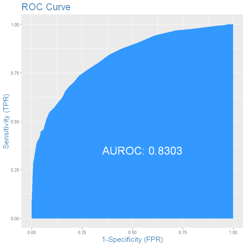
Побудуємо математичну модель:

h2o_model <- h2o.deeplearning(y = 'Exited', 
                              training_frame = as.h2o(train_data),
                              activation = "Rectifier",
                              hidden = c(6,6),
                              epochs = 100)

  |======================================================================| 100%
  |======================================================================| 100%

Варто перегляднути набір параметрів, що може приймати функція h2o.deeplearning(), адже вона досить складна:

# help(h2o.deeplearning) # можна переглянути параметри методу

Здійснимо прогноз на тестовій вибірці (h2o.predict()), а також класифікуємо значення за cutOff = 0.5:

h2o_predict_prob <- h2o.predict(h2o_model, newdata = as.h2o(test_data[-(ncol(test_data))]))

  |======================================================================| 100%
  |======================================================================| 100%

h2o_predict_class <- ifelse(h2o_predict_prob > 0.5, 1 , 0)
h2o_predict_class <- as.vector(h2o_predict_class)

Побудуємо матрицю Confusion Matrix:

suppressMessages(library(caret))
caret::confusionMatrix(factor(test_data$Exited), factor(h2o_predict_class), positive = "1")

Confusion Matrix and Statistics

          Reference
Prediction    0    1
         0 2285  104
         1  343  268
                                          
               Accuracy : 0.851           
                 95% CI : (0.8377, 0.8636)
    No Information Rate : 0.876           
    P-Value [Acc > NIR] : 1               
                                          
                  Kappa : 0.4624          
                                          
 Mcnemar's Test P-Value : <2e-16          
                                          
            Sensitivity : 0.72043         
            Specificity : 0.86948         
         Pos Pred Value : 0.43863         
         Neg Pred Value : 0.95647         
             Prevalence : 0.12400         
         Detection Rate : 0.08933         
   Detection Prevalence : 0.20367         
      Balanced Accuracy : 0.79496         
                                          
       'Positive' Class : 1               
                                          

Побудуємо ROC-криву:

library(InformationValue)
InformationValue::plotROC(test_data$Exited, as.vector(h2o_predict_prob))

Attaching package: 'InformationValue'


The following objects are masked from 'package:caret':

    confusionMatrix, precision, sensitivity, specificity

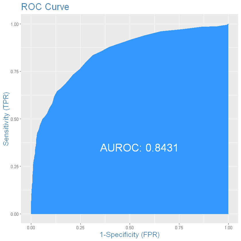
Побудуємо модель з більшою кількістю прихованих шарів та нейронів:

h2o_model2 <- h2o.deeplearning(y = 'Exited', 
                              training_frame = as.h2o(train_data),
                              activation = "Rectifier",
                              hidden = c(10,10),
                              epochs = 100)

  |======================================================================| 100%
  |======================================================================| 100%

Здійснимо прогноз:

h2o_predict_prob2 <- h2o.predict(h2o_model2, newdata = as.h2o(test_data[-(ncol(test_data))]))

  |======================================================================| 100%
  |======================================================================| 100%

h2o_predict_class2 <- ifelse(h2o_predict_prob2 > 0.5, 1 , 0)
h2o_predict_class2 <- as.vector(h2o_predict_class2)

Confiusion Matrix:

caret::confusionMatrix(factor(test_data$Exited), factor(h2o_predict_class2), positive = "1")

Confusion Matrix and Statistics

          Reference
Prediction    0    1
         0 2302   87
         1  343  268
                                         
               Accuracy : 0.8567         
                 95% CI : (0.8436, 0.869)
    No Information Rate : 0.8817         
    P-Value [Acc > NIR] : 1              
                                         
                  Kappa : 0.4765         
                                         
 Mcnemar's Test P-Value : <2e-16         
                                         
            Sensitivity : 0.75493        
            Specificity : 0.87032        
         Pos Pred Value : 0.43863        
         Neg Pred Value : 0.96358        
             Prevalence : 0.11833        
         Detection Rate : 0.08933        
   Detection Prevalence : 0.20367        
      Balanced Accuracy : 0.81263        
                                         
       'Positive' Class : 1              
                                         

ROC-крива:

InformationValue::plotROC(test_data$Exited, as.vector(h2o_predict_prob2))

Зупинимо двигун h2o:

h2o.shutdown(prompt = F)

---